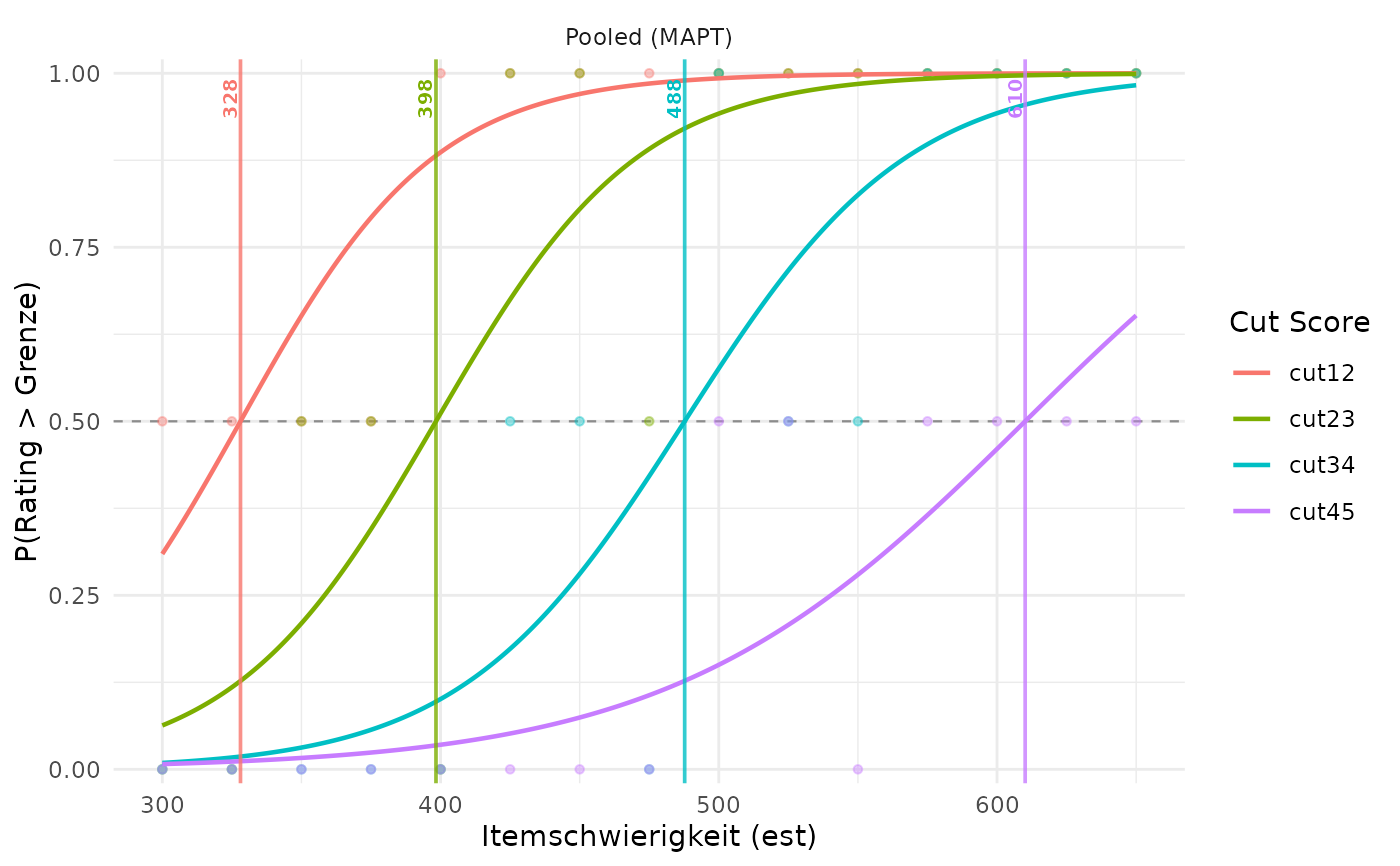
Plot IDM Cut Scores and Fitted Rating Functions

Shows how item ratings relate to item difficulty, and where the resulting cut scores lie. Pass the result of computeCutsIDM or computeCutsIDMMAPT directly to this function. Each rater gets a separate panel. show_aggregate = TRUE adds a summary panel: mean cuts for moving-average IDM, or a jointly fitted Pooled (MAPT) model for MAPT.

The y-axis depends on the method: rating levels for moving-average IDM, probabilities from zero to one for MAPT. Optional plausible values (PVs) add population distributions in the background and percentage tables above the panels. The background height is scaled for display; read population shares from the percentage tables, not from that height.

Usage

plotCutsIDM(
  res_list,
  est_col = NULL,
  show_raw = TRUE,
  show_smoothed = TRUE,
  show_residuals = FALSE,
  show_aggregate = FALSE,
  show_aggregate_labels = TRUE,
  show_cut_values = TRUE,
  show_item_numbers = TRUE,
  cut_value_digits = 0L,
  item_number_size = 2,
  cut_value_size = 2.6,
  aggregate_label_size = 3,
  pv_data = NULL,
  pv_cols = NULL,
  respondent_id_col = NULL,
  pv_id_col = NULL,
  pv_value_col = NULL,
  weight_col = NULL,
  input_format = c("auto", "long", "wide"),
  pv_missing = c("error", "drop"),
  density_bw = NULL,
  density_adjust = 1,
  population_height = 0.25,
  population_fill = "grey50",
  population_alpha = 0.15,
  population_col = NULL,
  population_colors = NULL,
  show_percentages = TRUE,
  percentage_digits = 1L,
  percentage_size = 3,
  show_population_stats = TRUE,
  population_stats_digits = 2L,
  show_caption = FALSE
)

Arguments

res_list: A result from computeCutsIDM() or computeCutsIDMMAPT(). The result's class selects the appropriate view.
est_col: Optional character scalar. Label to use for the item difficulty axis. If NULL, the value stored in res_list is used.
show_raw: Logical scalar. For moving-average IDM, shows raw ratings as points and a thin line connecting items ordered by difficulty. For MAPT, shows the empirical proportion of ratings above each boundary at each observed difficulty, within the relevant rater or pooled panel. MAPT points have the color of their boundary, matching its curve and cut line; see the worked example below. FALSE hides points but keeps the fitted MAPT curves.
show_smoothed: Logical scalar. Shows the non-monotonized moving average as a thin dashed blue line. Has no effect for MAPT results, whose logistic curves are always shown.
show_residuals: Logical scalar. Adds a residual row. For moving-average IDM, residuals are raw ratings minus smoothed moving averages. For MAPT, they are empirical proportions above each boundary minus the corresponding model probabilities at the same difficulties.
show_aggregate: Logical scalar. Adds a Mean panel for moving-average IDM, overlaying the monotonized rater curves and their mean cuts. For MAPT, adds a Pooled (MAPT) panel with the jointly fitted logistic curves and pooled cuts from res_list$cuts_summary. This is not a mean of the rater-specific cuts. If the MAPT result was computed with per_rater = FALSE, only the pooled panel is shown regardless of this option.
show_aggregate_labels: Logical scalar. Shows rater names near the right-hand end of monotonized curves in the Mean panel. Only used for moving-average IDM when show_aggregate = TRUE; has no effect for MAPT results.
show_cut_values: Logical scalar. If TRUE, numeric cut values are shown next to the vertical cut lines in individual panels and, when requested, in the aggregate panel.
show_item_numbers: Logical scalar. Shows item position numbers next to raw grey points in the individual moving-average IDM panels. Only used when show_raw = TRUE; has no effect for MAPT results.
cut_value_digits: Non-negative integer scalar. Number of digits after the decimal point used for rounding cut value labels. The default 0L shows rounded whole-number cut values.
item_number_size: Finite non-negative numeric scalar. Text size in millimetres for item position numbers next to raw points. Default is 2. Only used for moving-average IDM when show_raw = TRUE and show_item_numbers = TRUE.
cut_value_size: Finite non-negative numeric scalar. Text size in millimetres for numeric cut value labels in individual and aggregate panels. Default is 2.6. Only used when show_cut_values = TRUE.
aggregate_label_size: Finite non-negative numeric scalar. Text size in millimetres for rater names in the aggregate panel. Default is 3. Only used for moving-average IDM when show_aggregate = TRUE and show_aggregate_labels = TRUE.
pv_data: Optional wide- or long-format data frame of plausible values for one domain, optionally grouped into populations by population_col, already on the same metric as the item estimates and cuts. Supplying it adds background silhouettes to rating or MAPT probability panels. Default NULL leaves the plot unchanged. Silhouettes show distribution shape only; their height does not represent rating stages, rating probabilities, or density-axis values.
pv_cols: Character vector of PV column names, required for wide input. Wide input has one row per respondent. Other numeric columns are never selected automatically.
respondent_id_col: Optional respondent ID column, unique within each population for wide input; required for long input. IDs may repeat between populations. These are population respondent IDs, not rater IDs.
pv_id_col: PV identifier column for long input. Required together with pv_value_col and respondent_id_col. Each respondent-PV combination must be unique within its population.
pv_value_col: Numeric PV value column for long input.
weight_col: Optional sampling-weight column in pv_data. These weights affect population distributions, percentages, M, and SD. They do not change the rating models or cuts already stored in res_list. Default NULL uses equal weights. Weights must be finite, non-missing, non-negative, and constant across PVs for each respondent within its population. Zero-weight observations are excluded.
input_format: PV input layout. "auto" selects long format when pv_id_col or pv_value_col is supplied, and wide format otherwise.
pv_missing: Default "error" rejects missing PVs and omitted respondent-PV rows. "drop" omits them with a warning and renormalizes weights within each PV. Infinite PVs and invalid weights always cause an error. Every PV must retain at least two observed respondents with positive weights.
density_bw: Optional positive finite bandwidth in score units. Default NULL averages unweighted stats::bw.nrd0() bandwidths across PVs within each population, then averages those population means. All populations and PVs share this bandwidth. Sampling weights affect the density estimates, not automatic bandwidth selection.
density_adjust: Positive finite multiplier for the common density bandwidth. Default 1.
population_height: Finite fraction between zero and one of the rating- or probability-axis range occupied by the highest silhouette peak across all populations. Default 0.25. All silhouettes use the same height factor. This is a display setting for distribution shape only; silhouette height does not represent rating stages, rating probabilities, or density-axis values.
population_fill: Character vector of silhouette fill colors. An explicitly supplied single color applies to all populations. Otherwise supply exactly one color per observed population, in order of first appearance in the data (the population legend order); vector names are ignored. Too few or too many colors, including an empty vector, trigger a warning and restore the default colors. If omitted, ungrouped input uses "grey50"; grouped input uses the automatic palette described under population_colors. Explicit population_colors takes precedence.
population_alpha: Finite silhouette opacity between zero and one. Default 0.15.
population_col: Optional population grouping column in wide or long PV input. Labels must be non-missing and non-empty. Groups are drawn and listed in their order of first appearance; unused factor levels are ignored. Default NULL treats all rows as one population.
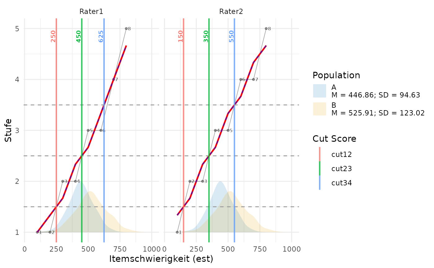
population_colors: Optional named character vector with exactly one color per observed population label. Requires population_col and takes precedence over population_fill. With neither color argument supplied, grouped input uses blue and orange for two groups (blue for one), or a qualitative palette for more groups. A separate population fill legend is added.
show_percentages: Logical scalar. Default TRUE adds percentage tables to rating panels when pv_data is supplied, with one colored row per population in legend order. Residual panels have no percentage labels. FALSE hides the tables and their additional caption. Has no plotting effect without pv_data.
percentage_digits: Integer scalar from zero to ten. Decimal places in percentage labels. Default 1L. Displayed totals can differ slightly from 100 percent because of rounding.
percentage_size: Finite non-negative percentage-table text size in millimetres. Default 3. Reduce this size or increase figure width for many intervals or small panels.
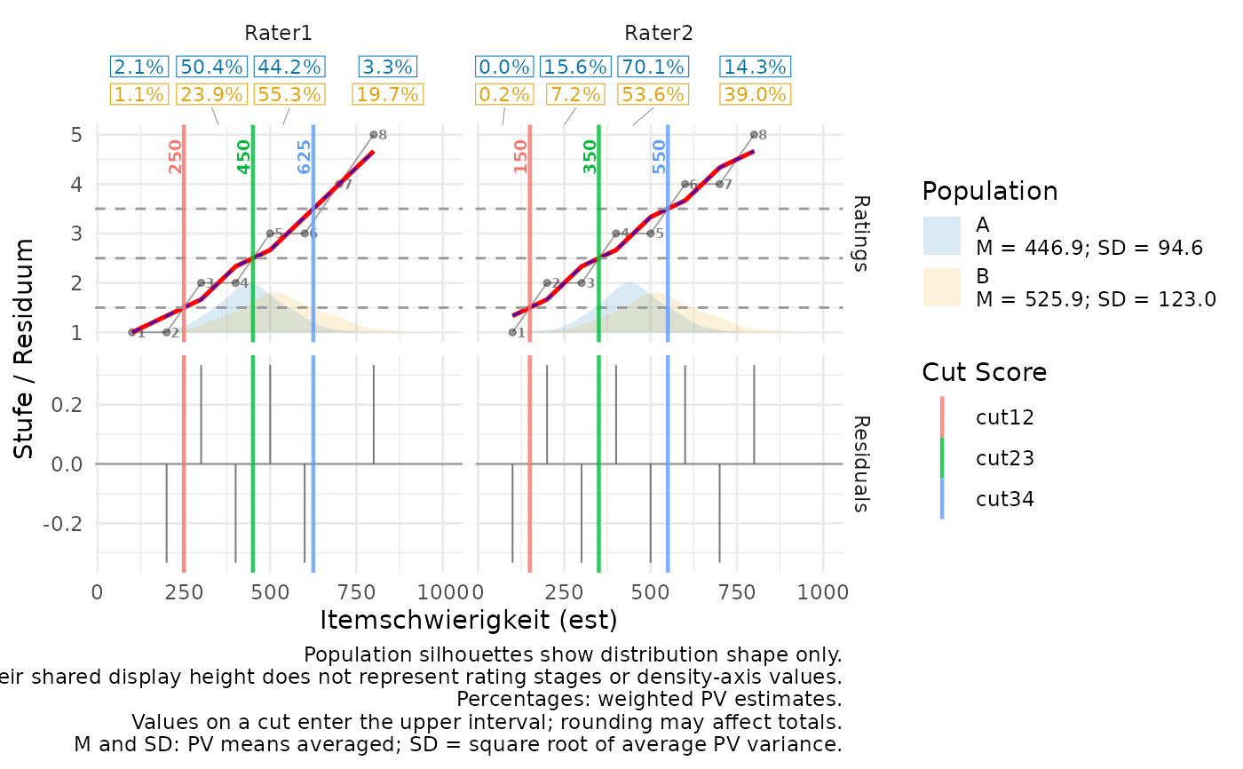
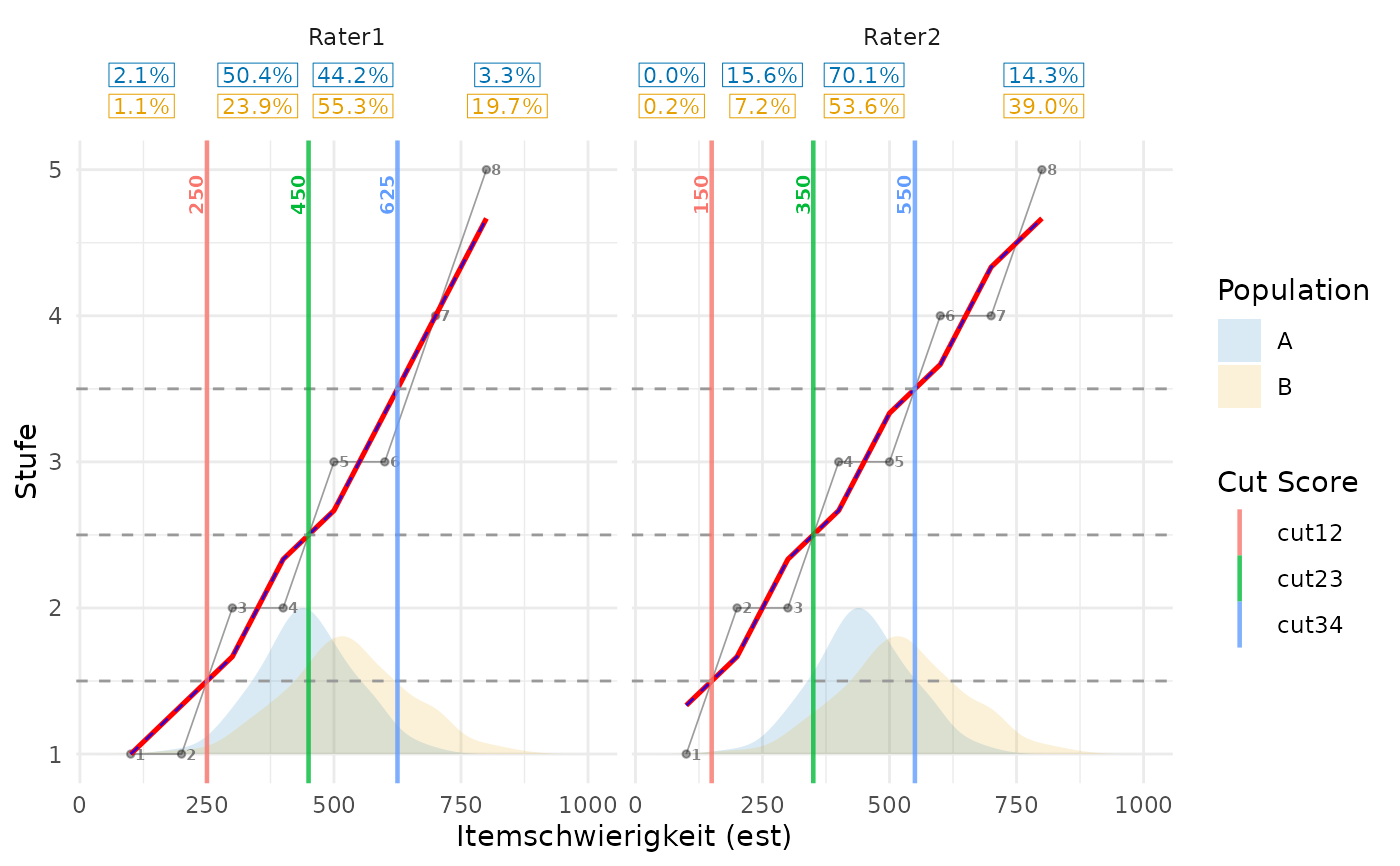
show_population_stats: Logical scalar. Default TRUE displays M and SD below each population name in the fill legend when pv_data is supplied. For ungrouped PV input they appear in the subtitle. FALSE hides these statistics and their caption line independently of show_percentages. Has no plotting effect without pv_data.
population_stats_digits: Integer scalar from zero to ten. Decimal places in displayed M and SD values. Default 2L. Use ggplot2::theme() to adjust legend.text or plot.subtitle text size.
show_caption: Logical scalar. Default FALSE hides explanatory plot captions. Set to TRUE to explain the population silhouette and, when displayed, percentages and M/SD below the plot. Does not affect statistics, percentage labels, or the subtitle. Has no plotting effect without pv_data.

Details

MAPT: read the axes and find a cut

This section applies to a result from computeCutsIDMMAPT(). The horizontal axis shows item difficulty on the original est scale. The vertical axis shows the probability of a rating above a selected boundary. For example, 0.75 means a fitted probability of 75 percent for that rating-level assignment. It is not a student's probability of answering the item correctly.

Rating labels first receive indices in the order given by rating_levels. For c("1a", "1b", "2", "3", "4"), those indices are 1, 2, 3, 4, 5. Thus, a boundary of 3.5 separates labels "2" and "3". The plotted cut, however, is an item difficulty such as 500; it is not 3.5.

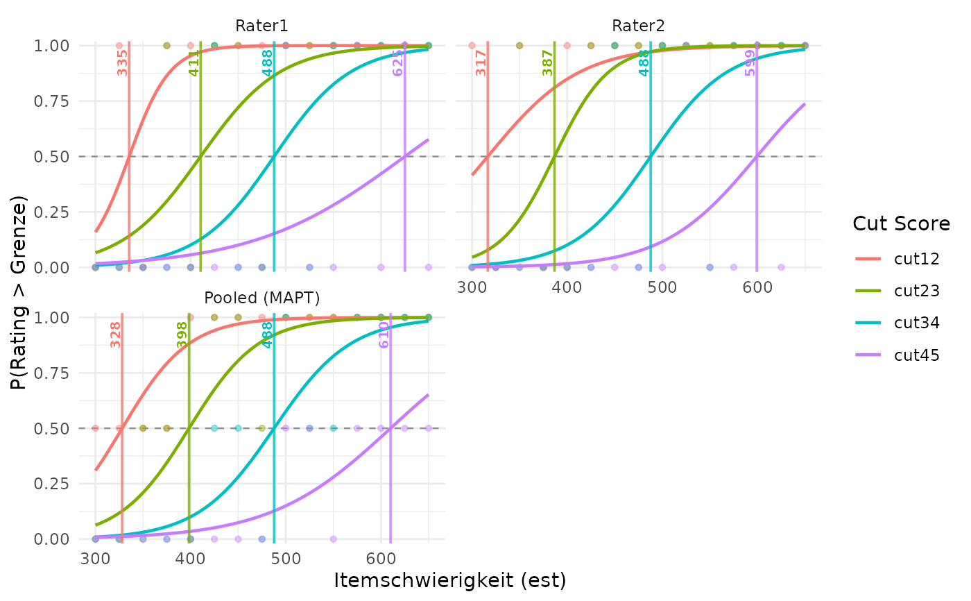
Each boundary has a fitted logistic curve: $$p_k(x)=\frac{1}{1+\exp[-(\alpha_k+\beta_k x)]}.$$ Here, $k$ identifies the boundary, $x$ is item difficulty, and $p_k(x)$ is the fitted probability of a rating above that boundary. The estimated intercept $\alpha_k$ and slope $\beta_k$ determine the position and steepness of the curve; $\exp$ is the exponential function.

To read the cut, find where the colored curve crosses the horizontal reference at 0.5. The vertical line of the same color marks that difficulty: $$p_k(c_k)=0.5, \qquad c_k=-\frac{\alpha_k}{\beta_k}.$$ For example, $\alpha_k=-10$ and $\beta_k=0.02$ give a cut of 500. The displayed number beside the cut line is rounded according to cut_value_digits; the line uses the unrounded cut.

Solid curves show predictions within the observed difficulty range of the panel. Dotted portions extend beyond that range: they are extrapolations.

MAPT: what the colored points mean

A color identifies a boundary. Points, the fitted curve, and the vertical cut line share that color. The legend shows which boundary each color represents. These colors do not identify individual items or raters, and are separate from the population colors used for PV backgrounds.

For each boundary, each observed rating contributes a zero or a one. A rating above the boundary contributes 1; a rating below it contributes 0. For example, a single rating of "2" in the five-level system above contributes the following four values:

Boundary between labels	Rating-index boundary	Value for rating `"2"`
`1a` and `1b`	1.5	1
`1b` and `2`	2.5	1
`2` and `3`	3.5	0
`3` and `4`	4.5	0

All four values have the same horizontal position: that item's difficulty. Several colors can therefore overlap at zero or one. Points are partly transparent, so overlapping colors can look like a mixed color. There is no single category color assigned to an item.

When several observations have exactly the same difficulty, the plot shows their mean zero-or-one value for each boundary. This is the observed proportion above that boundary. A point is therefore not always one item. For example, if three of four available ratings are above the boundary, the point is at $3/4=0.75$, even if the fitted curve is at 0.60.

More formally, let $A$ identify the panel (one rater, or all raters together). Let $S_A(x)$ be the set of observed item–rater pairs in that panel with difficulty exactly $x$, and let $n_A(x)$ be their number. The point height for boundary $b_k$ is $$q_{Ak}(x)=\frac{1}{n_A(x)} \sum_{(i,r)\in S_A(x)}\mathbf{1}(R_{ir}>b_k).$$ Here, $i$ identifies an item, $r$ a rater, and $R_{ir}$ is the rating index. The indicator $\mathbf{1}(\cdot)$ is 1 when its condition is true and 0 otherwise. Missing ratings are not counted. Different items with identical difficulties are combined in the same point; difficulties are not rounded or grouped into wider bins. Point size is constant and does not show how many ratings were combined. The models were fitted to the original rating observations, so a difficulty with more available ratings contributes more observations to the fit.

An individual rater panel uses only that rater's observations. The pooled panel counts all available observations at each difficulty together. It does not first average each rater's proportion and then average those proportions. For example, one rater contributing 1 upper-side rating out of 1 and another contributing 1 out of 3 give a pooled point at $(1+1)/(1+3)=0.5$.

Use show_raw = FALSE to hide the points when they obscure the curves. This changes the display only.

MAPT: individual panels, pooled panel, and residuals

Each individual panel uses that rater's fitted models and the cuts in cuts_per_person. With show_aggregate = TRUE, the additional Pooled (MAPT) panel uses the models jointly fitted to all ratings and the cuts in cuts_summary. A joint fit is not an average of the individual curves or cuts. cuts_summary_per_person, the optional mean of rater cuts, is not used in this plot. If the result was computed with per_rater = FALSE, the plot contains only the pooled panel, regardless of show_aggregate.

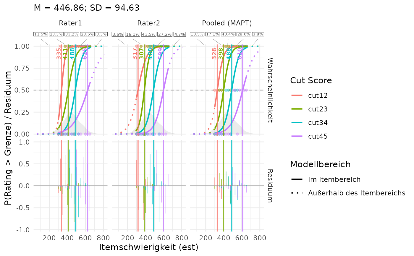
With show_residuals = TRUE, an additional row shows the differences between the observed proportions and the fitted probabilities: $$e_{Ak}(x)=q_{Ak}(x)-p_{Ak}(x).$$ Here, $A$, $k$, and $x$ identify the panel, boundary, and difficulty as above; $p_{Ak}(x)$ is the probability from that panel's model and $q_{Ak}(x)$ is its observed proportion. For example, $0.75-0.60=0.15$. A positive residual means more ratings were on the upper side than the model predicted; a negative residual means fewer. 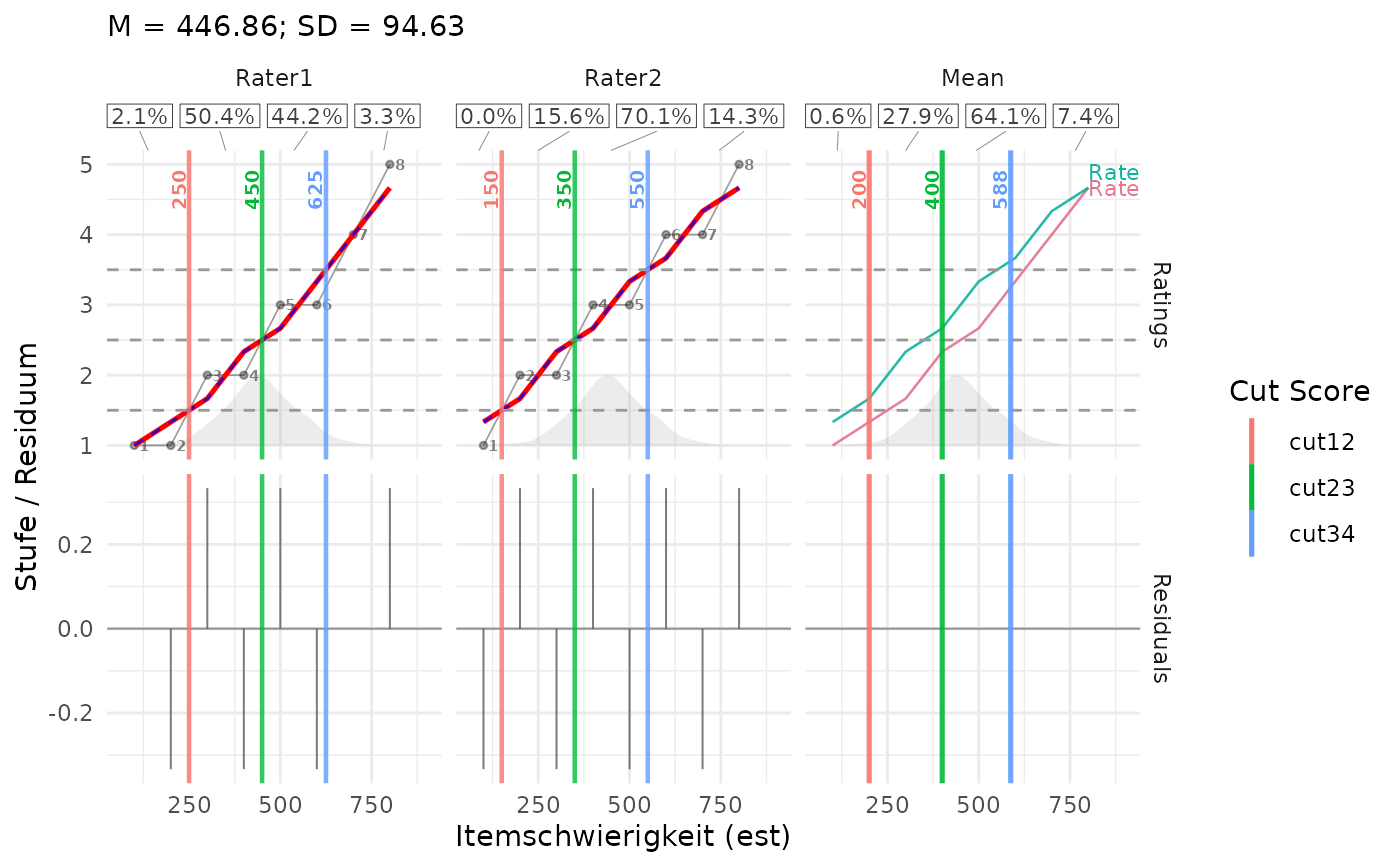Residuals are shown as vertical segments starting at zero. Cut lines repeat in the residual panels so their horizontal positions can be compared.

Only models with diagnostic status ok supply curves and residuals. Unusable fits have no cut line. A panel with no usable cuts remains visible with an explanatory label. See computeCutsIDMMAPT for the diagnostic meanings. Predictions use the stored models; for older results without individual model objects, the same curves are reconstructed from their diagnostic slopes and cuts. Plotting does not fit new models.

show_smoothed, show_item_numbers, and show_aggregate_labels apply only to moving-average IDM. They have no effect on MAPT plots; MAPT logistic curves are always shown.

Moving-average IDM: rating levels rather than probabilities

This section applies only to results from computeCutsIDM().

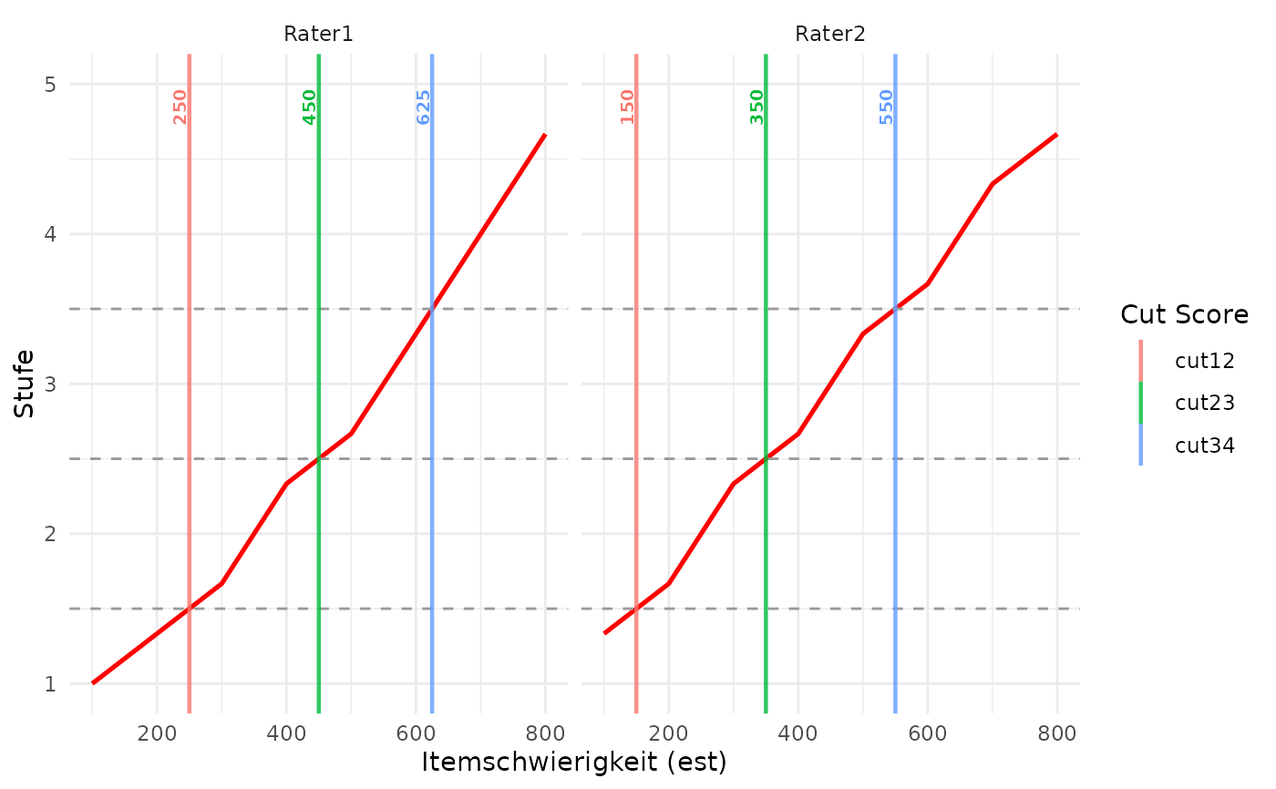
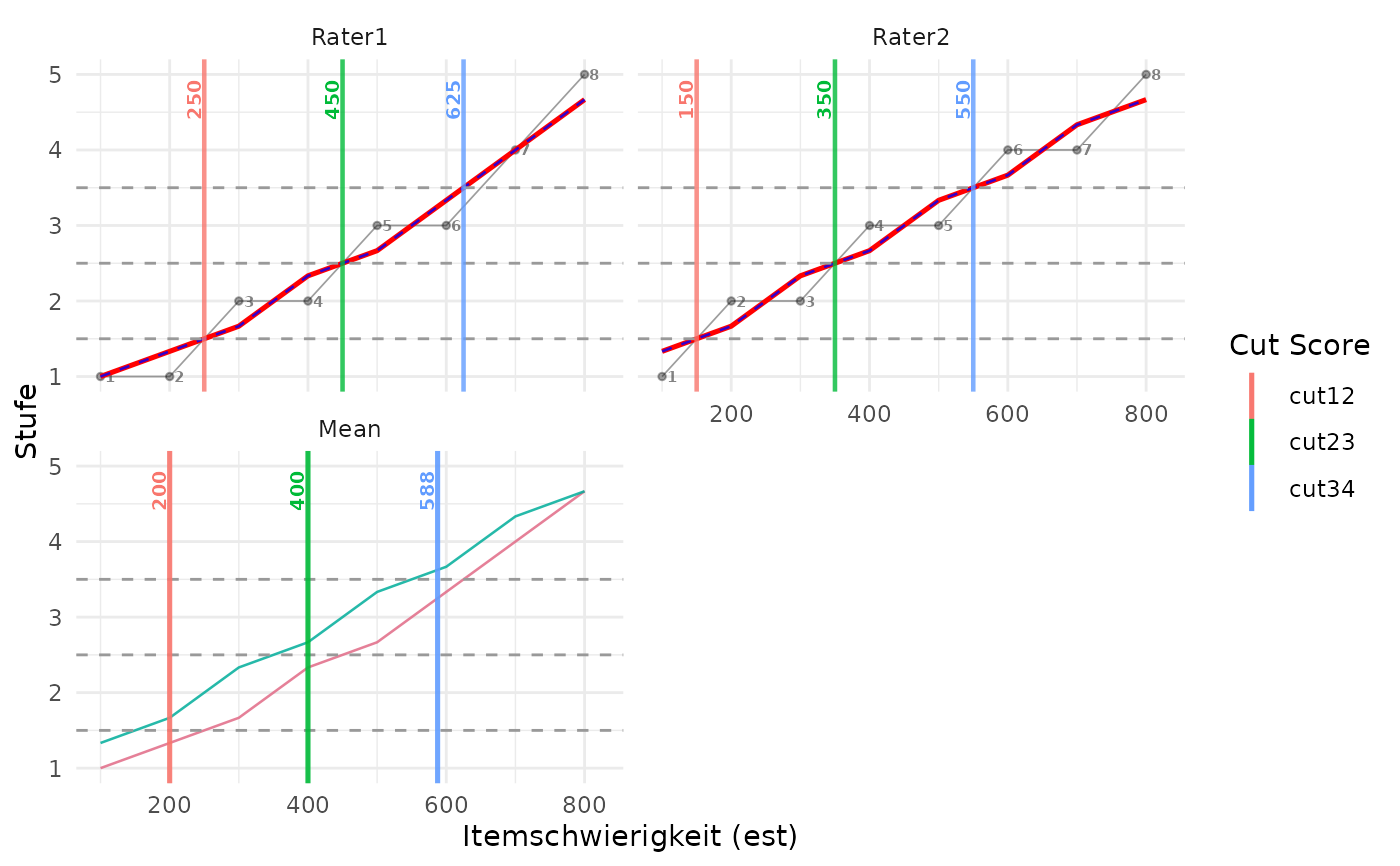
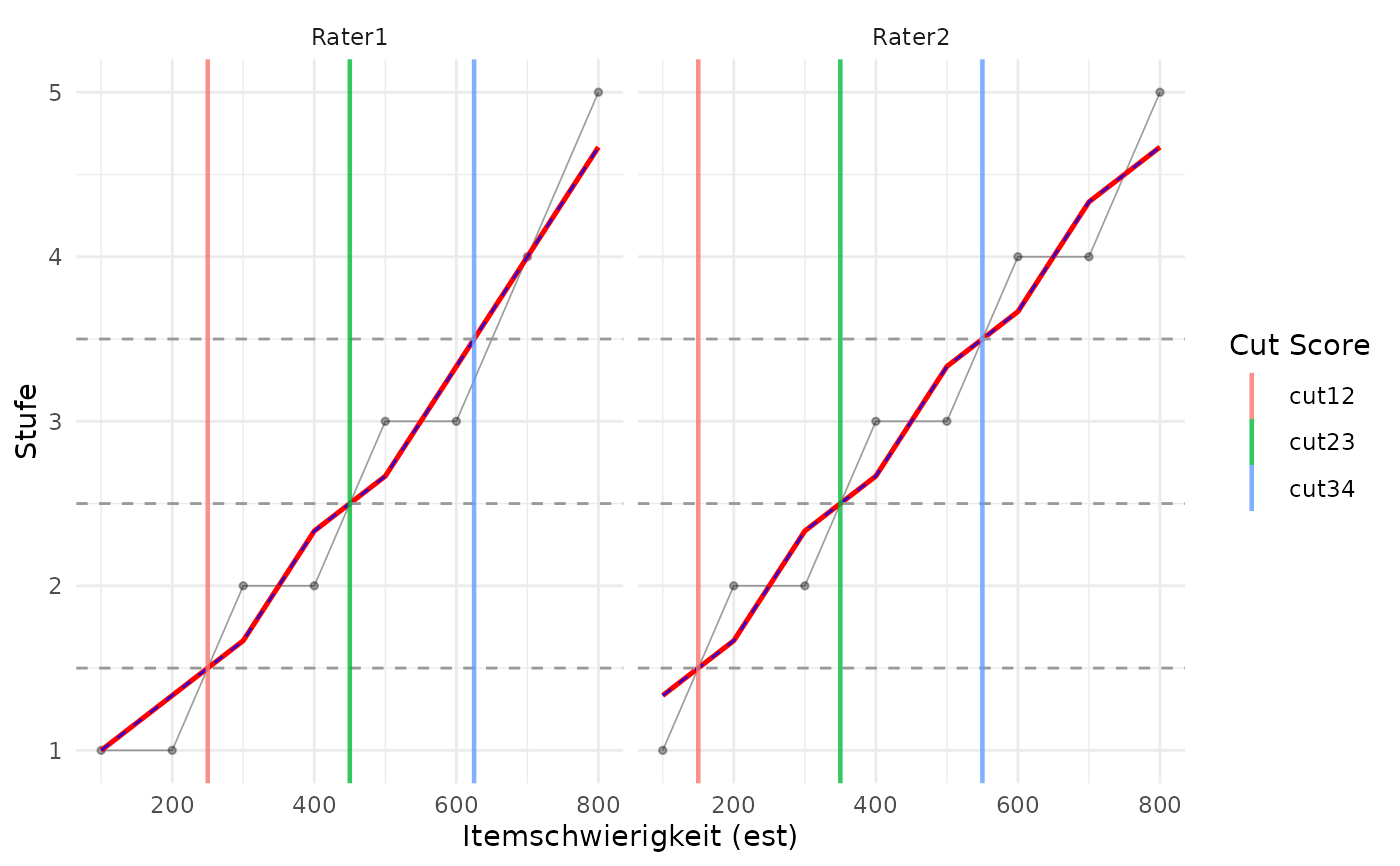
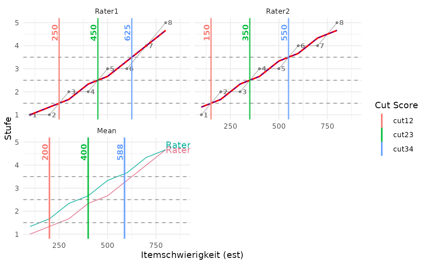
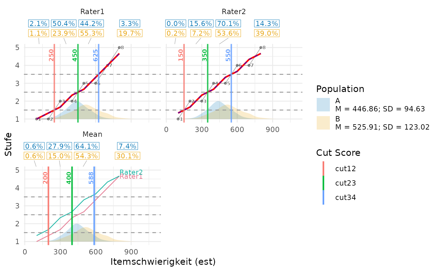
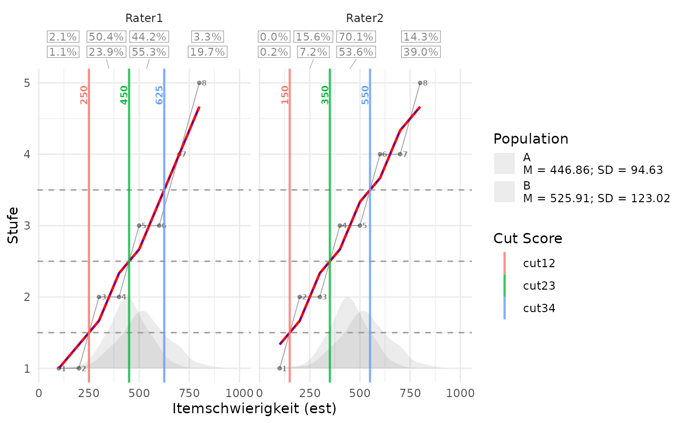
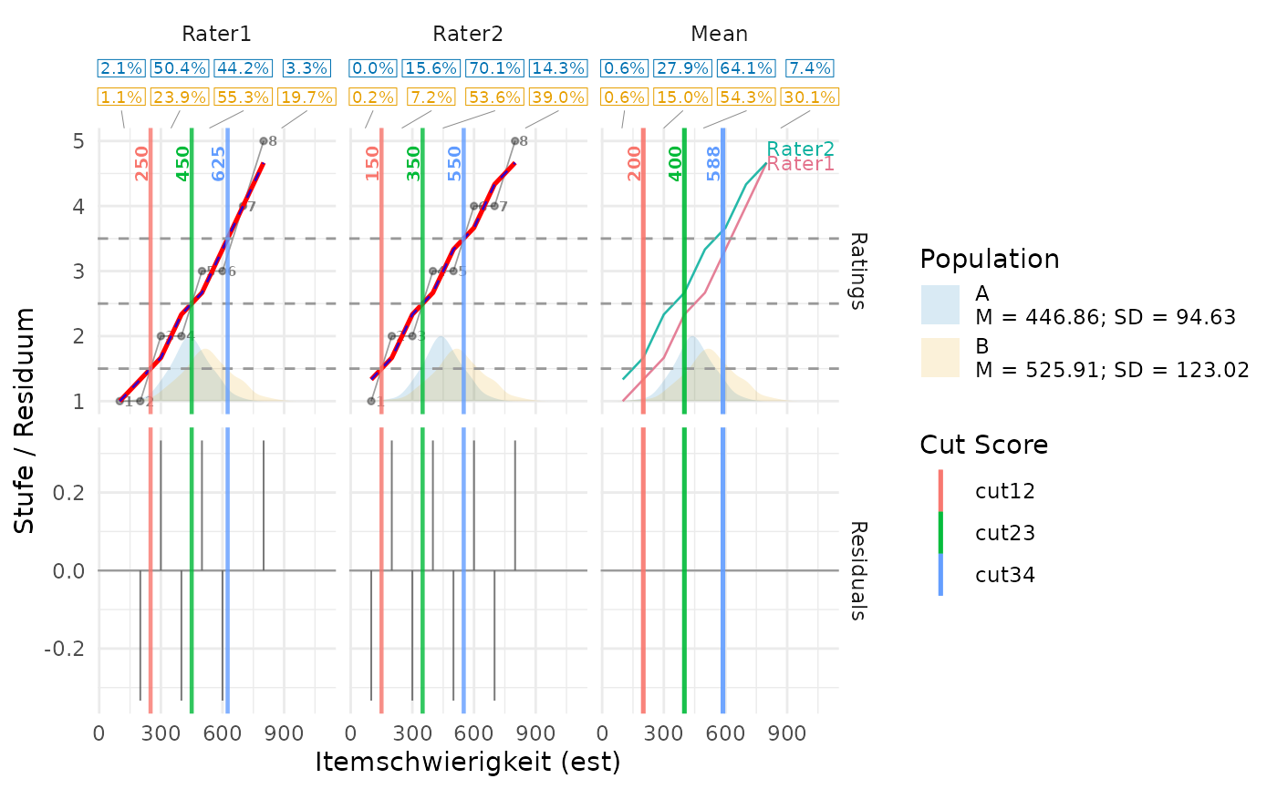
The y-axis shows rating levels. Grey points and a thin grey line show the original ratings, ordered by item difficulty. The dashed blue line shows a moving average, which smooths local variation. The red line shows the final isotonic curve: a version of the smoothed ratings that cannot decrease as difficulty increases. If the smoothed ratings are already non-decreasing, the blue and red lines coincide.

Horizontal lines mark rating boundaries. The vertical cut lines mark where the final red curve crosses those boundaries. The stored cuts use linear interpolation between neighboring points when needed. Use show_raw to control the grey points and line, and show_smoothed to control the blue line. The final red curve is always shown.

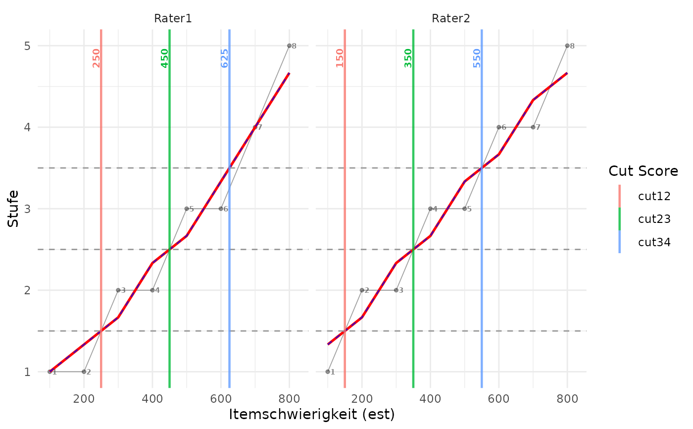
By default, the vertical cut lines are labelled with their numeric difficulty-scale values rounded to whole numbers. The number of digits after the decimal point can be changed with cut_value_digits. The grey raw-rating points in the individual rater panels are labelled with small item position numbers. These labels can be hidden with show_cut_values = FALSE and show_item_numbers = FALSE.

Technically, the plot is constructed from res_list$plot_data. For each rater facet, the x-axis is the item difficulty column stored as est; the y-values are the raw rating stage stage_raw, the smoothed moving average stage_sm, and the monotonized isotonic fit stage_iso. Horizontal lines are drawn at res_list$boundaries. Vertical lines are drawn at the difficulty-scale cuts in res_list$cuts_per_person; therefore the plotted cut positions are on the same x-axis scale as the item difficulties. Interpolated item positions, if needed for tabular summaries, are stored separately in res_list$cut_positions_per_person.

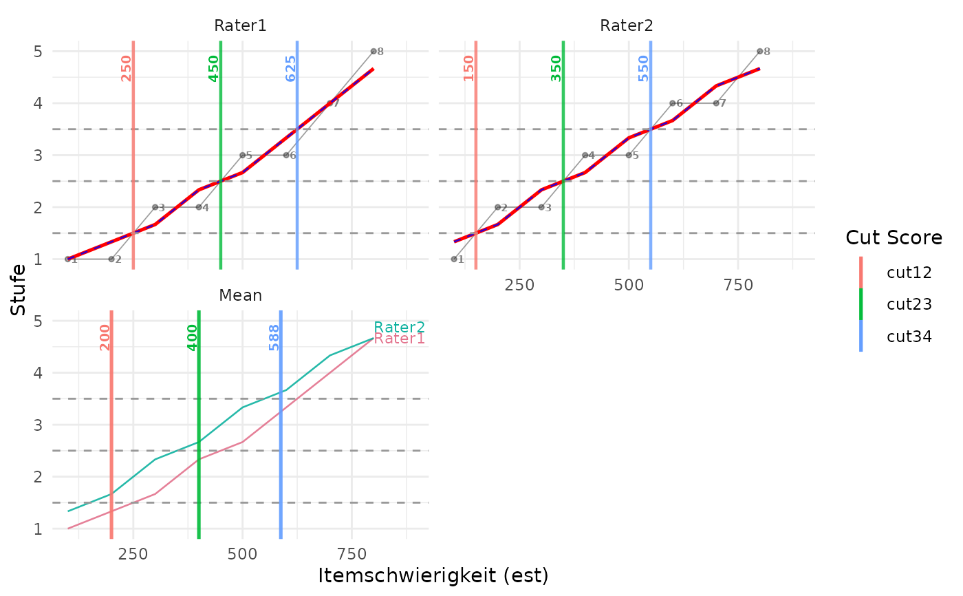
With show_aggregate = TRUE, the plot adds an aggregate panel labelled Mean. This panel overlays the monotonized rater curves from the individual panels as thin colored lines and draws vertical lines at the mean difficulty-scale cuts in res_list$cuts_summary. With show_aggregate_labels = TRUE, the colored curves are labelled by rater name near their right-hand end. Label positions are adjusted vertically when several rater curves end at similar values. These mean cuts correspond to the cut scores reported by summary(res_list). The color legend is reserved for cut score labels; aggregate rater colors are not added to the legend.

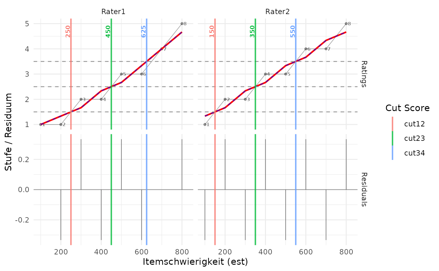
With show_residuals = TRUE, the plot uses an additional row of facets. The residual in item $i$ is $e_i = r_i - z_i$, where $r_i$ is the raw rating and $z_i$ is the smoothed moving average. Residuals are drawn as vertical segments from zero to $e_i$. The cut lines are repeated in the residual panel so that large local deviations can be inspected relative to the final cut locations.

If computeCutsIDM() stored ordinal rating labels in res_list, these labels are used on the y-axis.

Both methods: population backgrounds and their colors

Plausible values (PVs) are multiple draws of respondents' proficiency values. They describe a population of respondents, whereas the MAPT curves describe raters' level assignments to items. These are different sources of information. The PVs must already use the same score scale as the item difficulties and cuts.

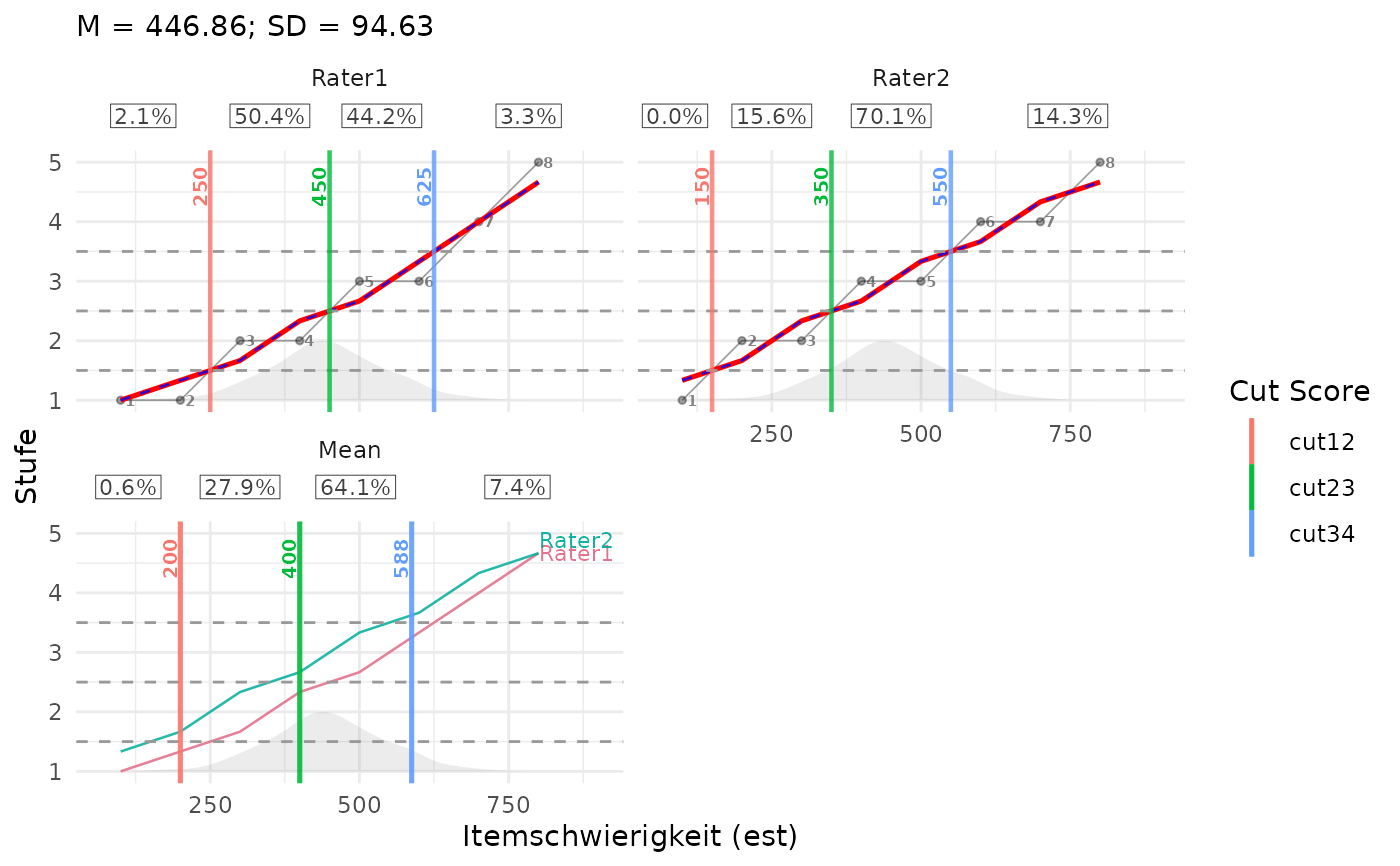
With pv_data, a population silhouette (a filled distribution shape) is drawn behind the curves and cut lines in every individual and aggregate main panel. It shows distribution shape only: its height is scaled for display and does not represent rating stages, rating probabilities, or density-axis values. An optional plot caption states this distinction when show_caption = TRUE; captions are hidden by default. The rating axis, curves, and cut calculations are unchanged; residual panels have no silhouette. The shared x-range expands to include the population density grid, so item curves may occupy a smaller portion of the plot.

The silhouette starts at the lower limit of the main y-axis: zero for MAPT. Its highest peak occupies population_height times that axis range. For MAPT, population_height = 0.5 places the highest peak at 0.5; this does not mean a 50-percent probability or population share. The same silhouette and scaling are used in every main panel. Gaussian densities are estimated separately for each PV using normalized sampling weights and then averaged on a common grid with a common bandwidth. Respondents' PVs are not averaged first. Population arguments are used only when pv_data is supplied.

With population_col, several silhouettes overlap transparently behind the same cuts and rater curves. Each population's density is computed and normalized separately using its own PVs and weights. All populations share one bandwidth and grid; weights and missing-data checks are handled within populations. Silhouettes are not stacked or separately stretched to equal peak heights. Instead, the largest density peak across all populations determines one shared display scaling factor, preserving relative differences in concentration. The fill legend identifies these populations; the cut-color legend identifies rating boundaries. Their colors have separate meanings. Background height shows distribution shape only and does not represent rating stages, rating probabilities, or density-axis values. Every main and aggregate panel repeats all populations with the same scaling; residual panels stay clear.

Both methods: what the percentage tables measure

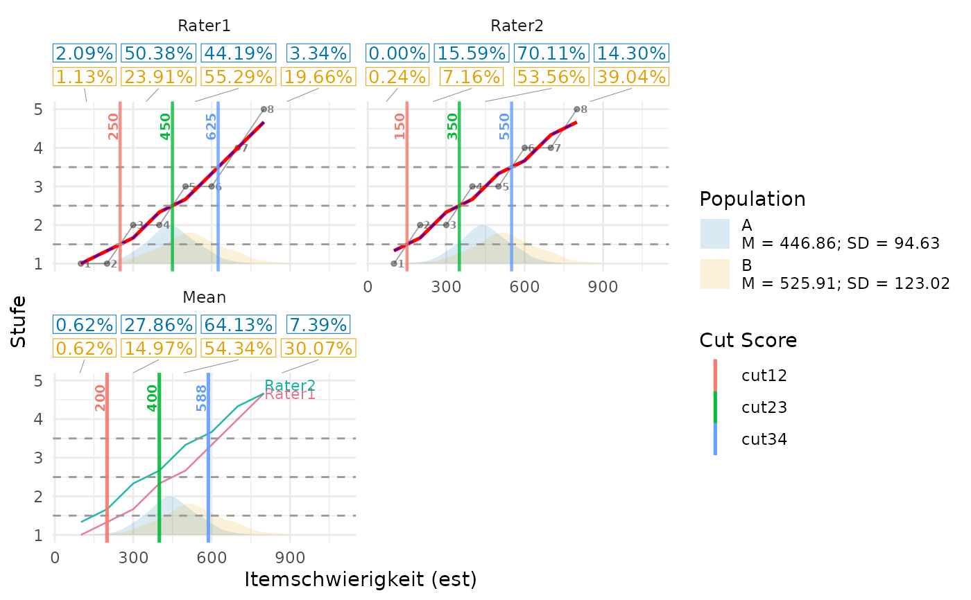
The percentage tables estimate how much of each respondent population falls between the cuts. This is different from the MAPT y-axis probability of a rating above a boundary. A population percentage is calculated from PVs and sampling weights, not from the height of a logistic curve.

For one population, the percentage in a score interval $C$ is $$S(C)=\frac{100}{M}\sum_{m=1}^{M} \frac{\sum_{j\in J_m} w_j\,\mathbf{1}(v_{jm}\in C)} {\sum_{j\in J_m} w_j}.$$ Here, $M$ is the number of PVs and $m$ identifies one PV. $j$ identifies a respondent, $v_{jm}$ is their value for PV $m$, and $w_j$ is their sampling weight (1 without weight_col). $J_m$ contains respondents with an observed value and positive weight for that PV. The indicator is 1 when the value lies in $C$, and 0 otherwise. The calculation is repeated separately for each population.

For example, if one interval contains 40 percent of the weighted observations for PV1 and 50 percent for PV2, the displayed estimate is $(40+50)/2=45$ percent. Respondents' PVs are not averaged before assigning them to intervals.

With two cuts $c_1<c_2$, the three intervals are $$(-\infty,c_1),\quad[c_1,c_2),\quad[c_2,\infty).$$ For example, with cuts 400 and 500, a score of 500 enters the last interval. Each individual panel uses its own rater's cuts. The MAPT pooled panel uses the jointly estimated cuts; the moving-average Mean panel uses mean cuts. Both aggregate panels recalculate percentages at their own cuts, rather than averaging individual raters' percentages.

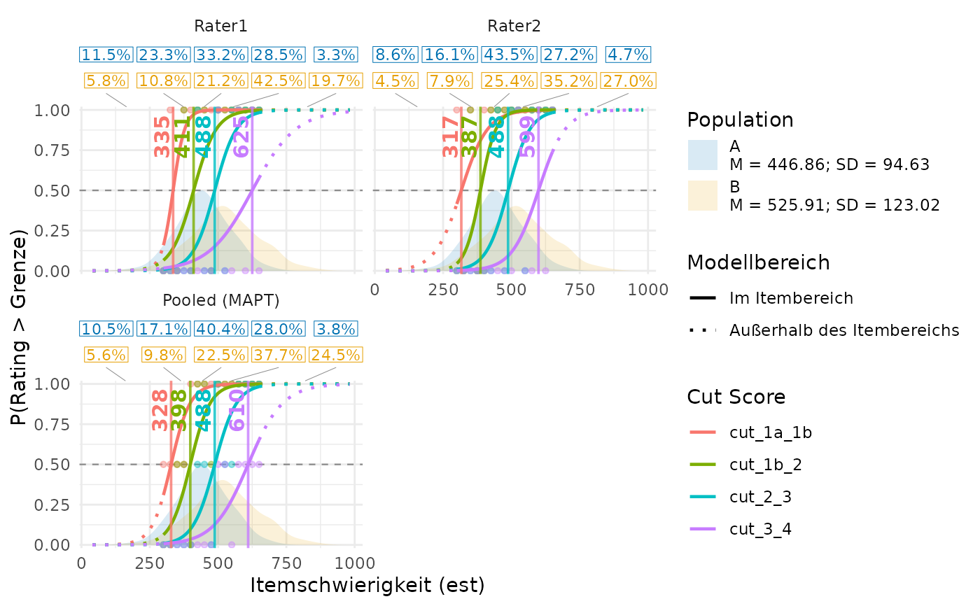
By default, each rating panel with population data also contains a percentage table. Percentage labels are centered between the visible cut positions; outer intervals use the midpoint between the outermost cut and the visible panel edge. Crowded labels shift as little as possible, preserving interval order, with thin lines connecting shifted columns to their interval midpoints. Population rows stay horizontally aligned. Placement uses rendered text widths and adapts to resizing, zooming, and reversed score axes. Intervals wholly outside a zoomed view are anchored at its edge, with their percentages unchanged. Each population has a separate row, following the population legend's order and colors. Each table occupies a separate band above the data, with height determined by its text size and number of rows. The data axes are unchanged, and the tables stay clear of rating curves when the figure is resized. Increase figure height for many panels or populations, and figure width for many intervals. Residual panels receive no percentage labels. If the combined label widths exceed the panel width, text and padding are reduced together to fit; increase figure width to retain the requested text size.

Percentages are calculated directly from PVs and sampling weights, separately for every population and PV, then averaged equally across PVs. Available weights are normalized within each PV after the selected missing-data handling. Values exactly on a cut belong to the upper interval. The two outer intervals extend to infinity, so observations outside the visible x-range are included. Identical cuts create empty intervals with zero percent. Actual unrounded cuts are used: cut-label rounding, density smoothing, and population_height do not affect percentages. A panel with missing or infinite cuts displays an explanatory message instead of partial percentages and triggers a warning; descending cuts cause an error when percentages are enabled.

Percentage labels are estimated population shares. Silhouette height still shows distribution shape only and does not represent rating stages, rating probabilities, or density-axis values. Set show_caption = TRUE to include this explanation.

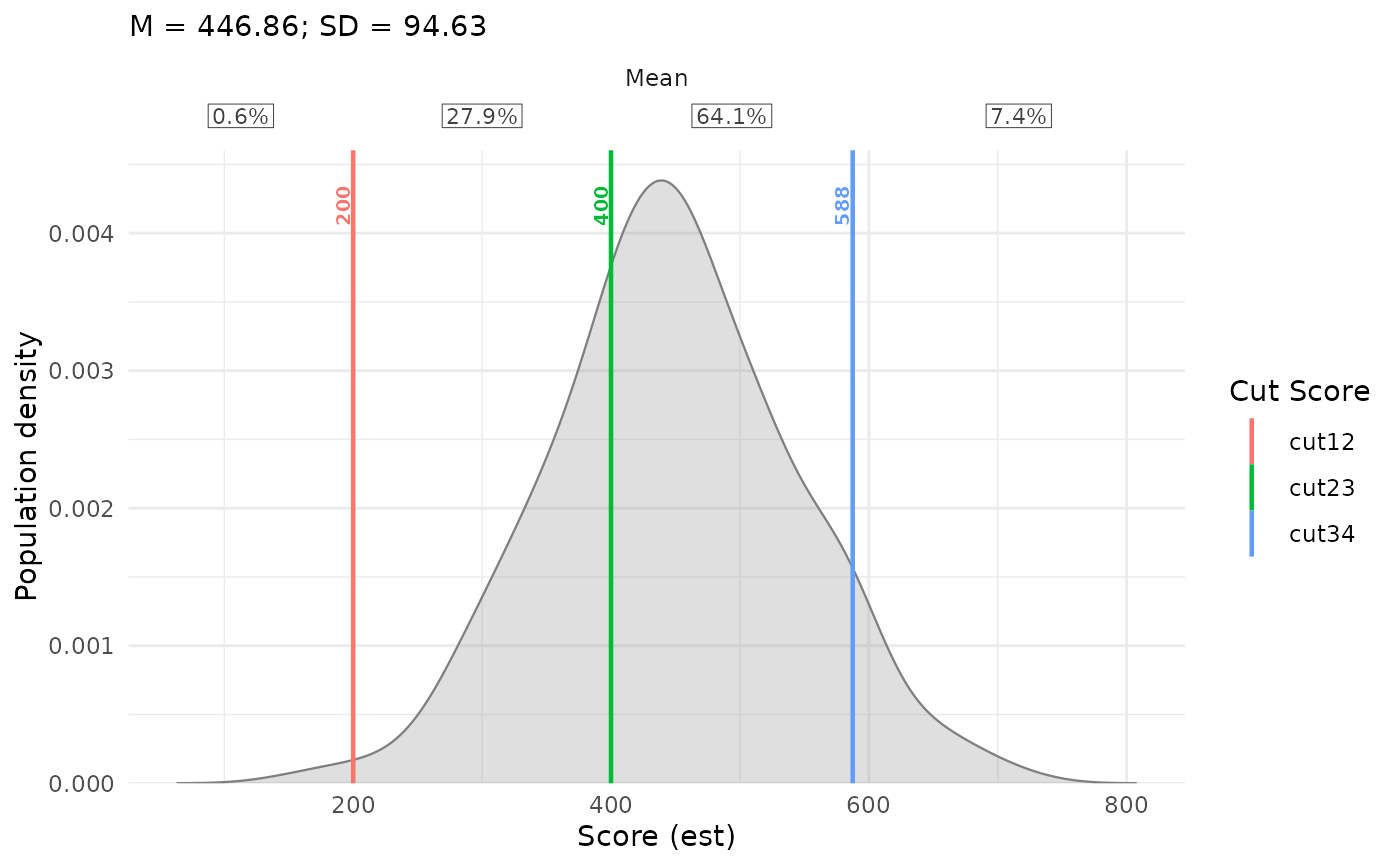
See plotPopulationCutsIDM for the same distribution with a real density axis, full details of PV processing, and wide- and long-format examples. Both views are descriptive estimates and do not calculate uncertainty intervals. If cuts are out of order, use show_percentages = FALSE to inspect the curves without attempting to calculate population shares.

Both methods: population mean and spread

M is the population mean and SD is the population standard deviation, a measure of spread on the score scale. They describe the respondents, not agreement between raters or the uncertainty of a cut.

With population data, M and SD are shown by default using the same computation as plotPopulationCutsIDM(): M averages the weighted PV means, and SD is the square root of the average weighted PV variance, with an $n/(n-1)$ correction applied separately within each PV and population. Here, $n$ is the number of respondents with an observed value and positive weight for that PV and population. See its details for the formula and weighting convention. The statistics describe each whole population on the supplied score metric and are shared across individual and aggregate panels, including plots with residual panels. They are independent of cuts, density smoothing, and silhouette height. Silhouette height still communicates distribution shape only and does not represent rating stages, rating probabilities, or density-axis values.

Value

A ggplot2 object.

Examples

dat <- data.frame(
  est = seq(100, 800, by = 100),
  Rater1 = c(1, 1, 2, 2, 3, 3, 4, 5),
  Rater2 = c(1, 2, 2, 3, 3, 4, 4, 5)
)

res <- computeCutsIDM(dat, boundaries = c(1.5, 2.5, 3.5))
plotCutsIDM(res)


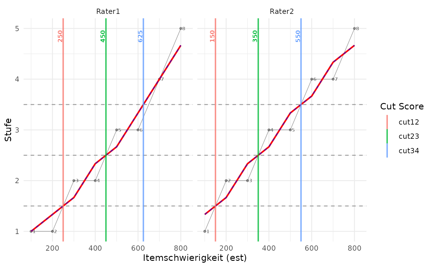## The plotted vertical lines correspond to these difficulty-scale cuts:
res$cuts_per_person
#> # A tibble: 2 × 4
#>   person cut12 cut23 cut34
#>   <chr>  <dbl> <dbl> <dbl>
#> 1 Rater1   250   450   625
#> 2 Rater2   150   350   550

## Hide the auxiliary raw and smoothed functions:
plotCutsIDM(res, show_raw = FALSE, show_smoothed = FALSE)


## Add an aggregate panel with all monotonized curves and mean cuts:
plotCutsIDM(res, show_aggregate = TRUE)


## Hide rater labels in the aggregate panel:
plotCutsIDM(res, show_aggregate = TRUE, show_aggregate_labels = FALSE)


## Hide cut value and item number labels:
plotCutsIDM(res, show_cut_values = FALSE, show_item_numbers = FALSE)


## Show cut value labels with two digits after the decimal point:
plotCutsIDM(res, cut_value_digits = 2)


## Add residual panels:
plotCutsIDM(res, show_residuals = TRUE)


## Enlarge the labels inside the graph:
plotCutsIDM(res, show_aggregate = TRUE,
            item_number_size = 3, cut_value_size = 3.5,
            aggregate_label_size = 4)


## Synthetic PVs on the item-estimate and cut metric.
set.seed(42)
population <- data.frame(
  student = seq_len(200),
  PV1 = rnorm(200, 450, 100),
  PV2 = rnorm(200, 450, 100),
  weight = runif(200, 0.5, 2)
)

## Silhouette = distribution shape only; height does NOT represent rating stages.
## Use show_caption = TRUE to include the silhouette explanation below the plot.
plotCutsIDM(res, pv_data = population, pv_cols = c("PV1", "PV2"),
            weight_col = "weight", show_aggregate = TRUE,
            population_height = 0.25, population_alpha = 0.15)


## The same shape-only silhouette stays out of residual panels.
population_long <- tidyr::pivot_longer(
  population, cols = c("PV1", "PV2"),
  names_to = "pv", values_to = "score"
)
plotCutsIDM(res, pv_data = population_long,
            respondent_id_col = "student", pv_id_col = "pv",
            pv_value_col = "score", weight_col = "weight",
            show_aggregate = TRUE, show_residuals = TRUE)


## Use a standalone plot when the density axis is needed.
plotPopulationCutsIDM(res, population, pv_cols = c("PV1", "PV2"),
                      weight_col = "weight")


## Two populations with a shared silhouette-height factor, not rating values.
population$group <- "A"
population_b <- population
population_b$group <- "B"
population_b[c("PV1", "PV2")] <- 450 +
  1.3 * (population_b[c("PV1", "PV2")] - 450) + 80
populations <- rbind(population, population_b)
plotCutsIDM(res, pv_data = populations, pv_cols = c("PV1", "PV2"),
            respondent_id_col = "student", weight_col = "weight",
            population_col = "group",
            population_colors = c(A = "#0072B2", B = "#E69F00"),
            population_alpha = 0.2, show_aggregate = TRUE)


## One explicit fill color applies to all population silhouettes.
plotCutsIDM(res, pv_data = populations, pv_cols = c("PV1", "PV2"),
            weight_col = "weight", population_col = "group", population_fill = "grey50")

## Or use population_fill = c("#009E73", "#CC79A7") in population legend order.
## Three colors for these two groups would warn and restore the default palette.

## Long input and residuals: silhouettes still show distribution shape only.
populations_long <- tidyr::pivot_longer(
  populations, cols = c("PV1", "PV2"), names_to = "pv", values_to = "score"
)
plotCutsIDM(res, pv_data = populations_long, respondent_id_col = "student",
            pv_id_col = "pv", pv_value_col = "score", weight_col = "weight",
            population_col = "group", show_aggregate = TRUE, show_residuals = TRUE)


## Percentages are population shares; silhouette heights are display-only.
plotCutsIDM(res, pv_data = populations, pv_cols = c("PV1", "PV2"),
            weight_col = "weight", population_col = "group",
            show_aggregate = TRUE, percentage_digits = 2, percentage_size = 3.5)


## Keep silhouettes and cut labels, but hide the percentage tables.
plotCutsIDM(res, pv_data = populations, pv_cols = c("PV1", "PV2"),
            weight_col = "weight", population_col = "group", show_percentages = FALSE)


## M and SD use the same population legend as plotPopulationCutsIDM().
plotCutsIDM(res, pv_data = populations, pv_cols = c("PV1", "PV2"),
            weight_col = "weight", population_col = "group",
            show_residuals = TRUE, population_stats_digits = 1, show_caption = TRUE)


## Hide M and SD independently of interval percentages.
plotCutsIDM(res, pv_data = populations, pv_cols = c("PV1", "PV2"),
            weight_col = "weight", population_col = "group", show_population_stats = FALSE)


## MAPT logistic curves use a probability axis and cuts at probability 0.5.
## Overlapping ratings avoid perfect separation in this example.
mapt_dat <- data.frame(
  est = seq(300, 650, length.out = 15),
  Rater1 = c(1, 2, 1, 3, 2, 4, 3, 2, 5, 3, 4, 5, 4, 5, 4),
  Rater2 = c(2, 1, 3, 1, 2, 3, 4, 3, 4, 5, 3, 4, 5, 4, 5)
)
mapt <- computeCutsIDMMAPT(mapt_dat)
plotCutsIDM(mapt, show_aggregate = TRUE)


## Hide overlapping boundary-colored points; retain curves and cut lines.
plotCutsIDM(mapt, show_aggregate = TRUE, show_raw = FALSE)


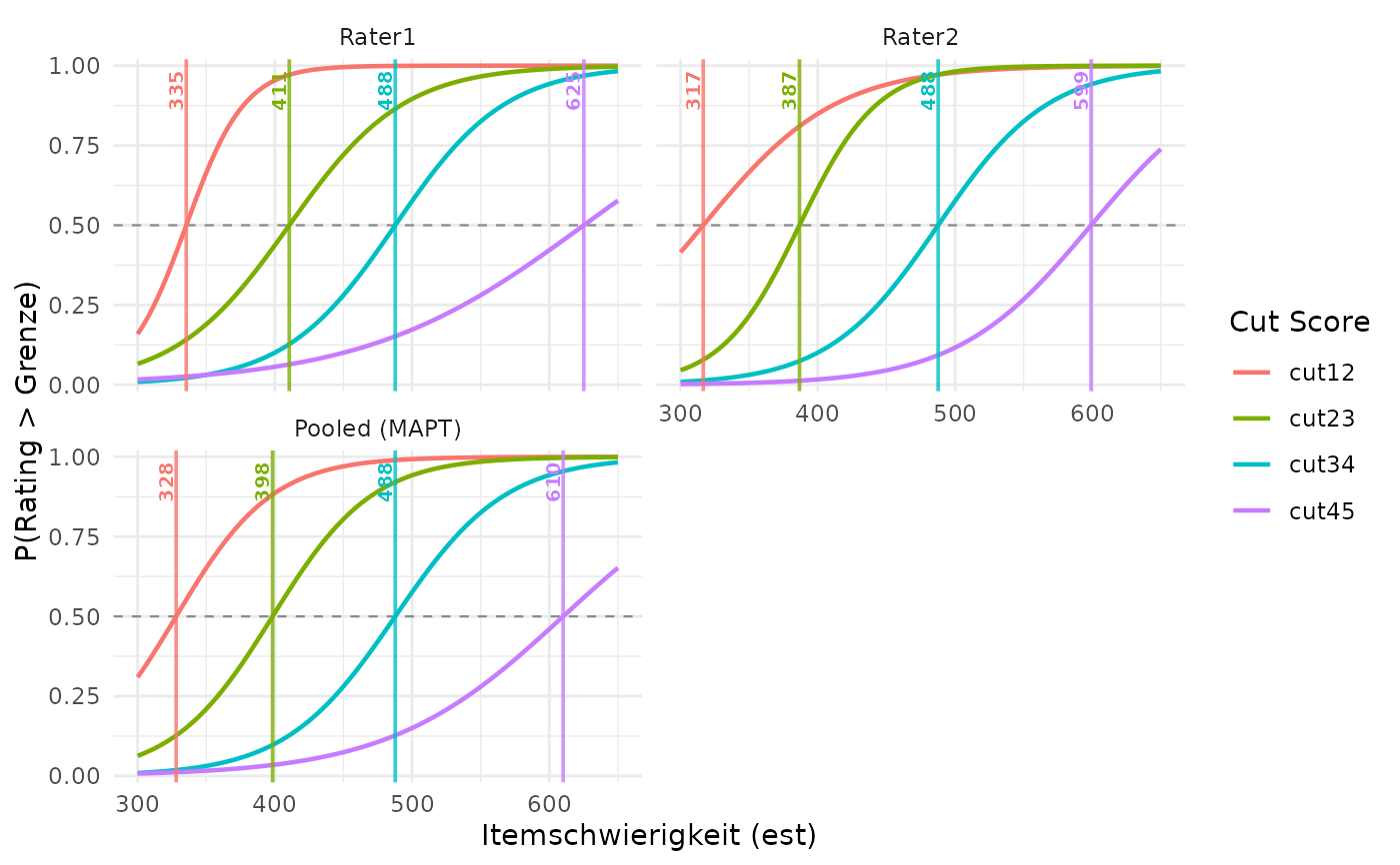## Use the level names in the cut legend.
level_labels <- c("1a", "1b", "2", "3", "4")
labelled_dat <- mapt_dat
labelled_dat$Rater1 <- level_labels[labelled_dat$Rater1]
labelled_dat$Rater2 <- level_labels[labelled_dat$Rater2]
labelled_mapt <- computeCutsIDMMAPT(labelled_dat, rating_levels = level_labels)
plotCutsIDM(labelled_mapt, show_aggregate = TRUE)


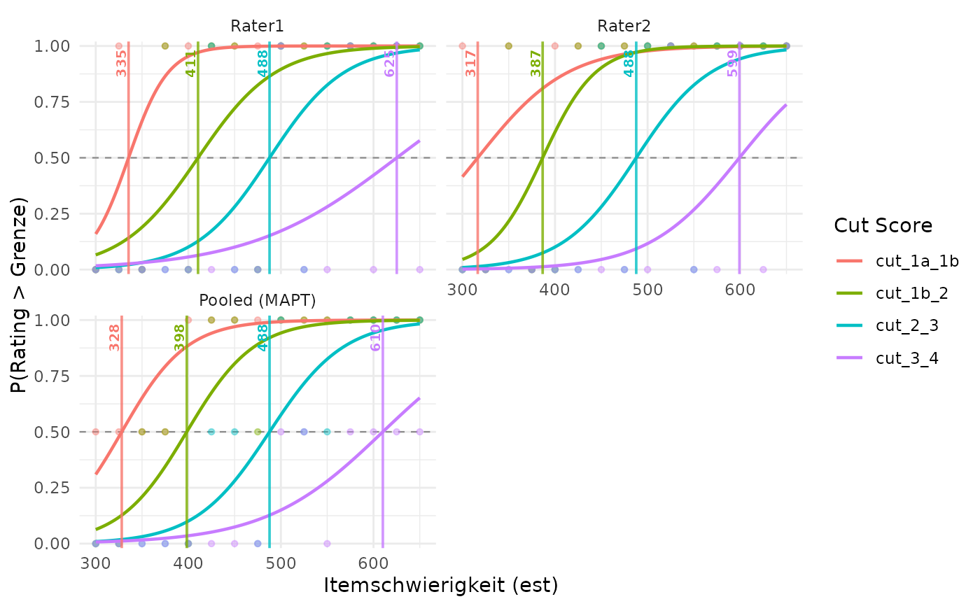## All rater panels and the pooled panel show both respondent populations.
## The 0.5 background height is a display setting, not a population share.
plotCutsIDM(labelled_mapt, show_aggregate = TRUE,
            pv_data = populations, pv_cols = c("PV1", "PV2"),
            weight_col = "weight", population_col = "group",
            population_height = 0.5, cut_value_size = 4, percentage_size = 4)


## Pooled curves/cuts are jointly estimated, not averaged across raters.
## PV silhouette height shows distribution shape, not rating probability.
plotCutsIDM(mapt, show_aggregate = TRUE, show_residuals = TRUE,
            pv_data = population, pv_cols = c("PV1", "PV2"),
            weight_col = "weight")


## Without individual models, the plot shows only the pooled panel.
plotCutsIDM(computeCutsIDMMAPT(mapt_dat, per_rater = FALSE))