Getting Started

Installation

eatPrep is on GitHub. You can install R packages from GitHub via the remotes package. With the following code you can download both packages remotes and eatPrep.

#install.packages("remotes")
#remotes::install_github("https://github.com/sachseka/eatPrep")
library(eatPrep)
#> Loading required package: readxl

Introduction

The goal of eatPrep, short for Educational Assesment Tools: Preparation, is to automate the preparation of item response test data; especially but not exclusively for typical use cases at the Institute for Educational Quality Improvement (IQB). Therefore it works together with IQB-specific applications such as the ItemDB or ZKDaemon.

Paper Competence Data Preparation

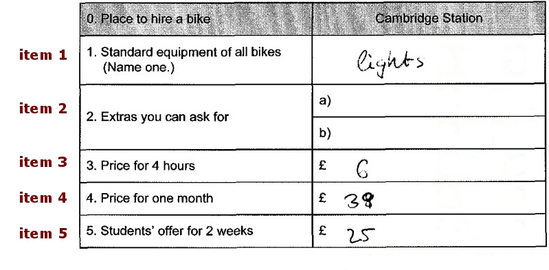
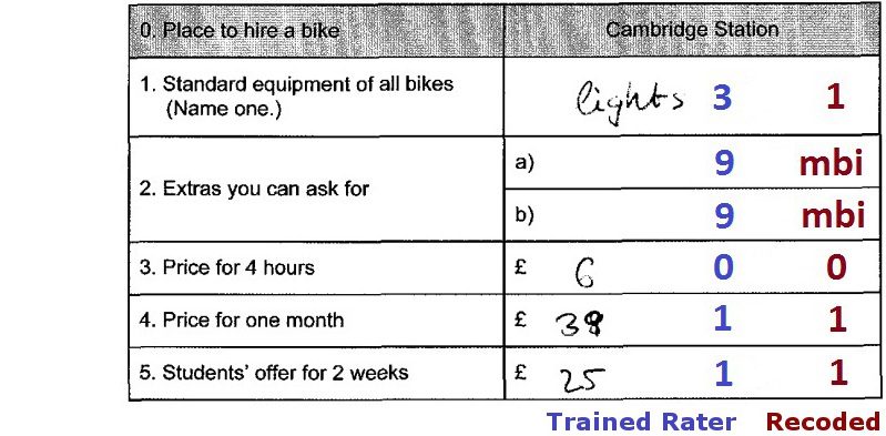
We usually give students paper tests or questionnaires that they fill out by hand, while being supervised. The results are later collected centrally. These tests are then scanned. For multiple choice questions or tick questions an optic scanning system is used that recognizes marked fields automatically and transmits them to a digital data bank. Trained coders evaluate the (partially) open questions. This data is usually in a SPSS (.sav) format.

We use eatPrep for the standardization and automation of the handling of such data.

Features

The main purpose of eatPrep is to read, score, aggregate and merge data from a regular SPSS (.sav) data file (via the function readSpss()) and meta data from databases (readDaemonXlsx()) and Excel spreadsheets (readMerkmalXlsx()). Additional functions include checking the data (checkData()), meta data (checkInputList()), and the design (checkDesign()), recoding of (missing) values (recodeData(), mnrCoding(), aggregateData(), scoreData(),collapseMissings()), working with rater data (meanAgree(), meanKappa()), evaluating item categories (catPbc(), evalPbc()) and exporting prepared or raw item data sets to different formats (writeSpss(), prep2GADS()). Most of this can be done with a single function call to automateDataPreparation().

Automation of Data Preparation

Various tests, plausibility checks and diagnostics

Handling of many different missing types, if desired retention until the end (incl. missing-not-reached calculation)

Additional tools (category separation, rater functions, semi-manual data cleansing, export functions…)

Data Structures of Paper Competency Data at the IQB

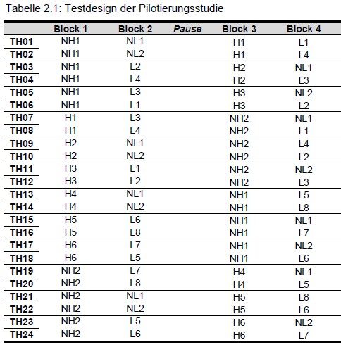
In a prototypical scenario, we are constructing a test at the IQB, e.g. for educational purposes. For our pilot study, we have created several overlapping booklets and a variety of items with different item formats (constructed response, multiple choice).
Thereby, the data consists of several layers:

booklets	containing blocks
blocks/cluster	containing tasks
tasks	contain units (=items) (usually for a common stimulus/testlet)
units	containing subunits/subitems
subunits	having values
values	including missings and recode values
valueRecodes	also “Scores”: A mapping of the original values to a smaller number of categories (usually at least True/False/Missing, i.e. 1/0/NA) that are better suited for IRT scaling

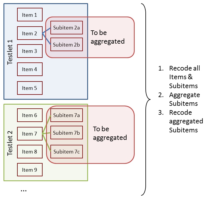
The goal is to:

1. Recode all items and subitems
2. Aggregate subitems
3. Recode aggregated subitems

Subitems, Items and Tasks	Subitems, Items, Tasks, Values and Scores

Tasks in blocks and blocks in booklets

Missing Values

Now we would like to prepare the data collected in this way for scaling. In doing so, we would like to know if the booklets are speeded (number of mnr). Additionally, we intend to use different missing treatments for the actual scaling, so we preserve missing values during data preparation and recode them right before scaling the data. eatPrep can help us with all of that.

Here is an overview for different value types the IQB uses:

Missing Types

Code	Label	Abbr	Explanation
-98	mir	missing invalid response	(1) Item was edited, and (2a) empty answer or (2b) invalid (joke) answer.
-99	mbo	missing by omission	Item wasn’t edited but seen, or wasn’t seen, but there are seen or edited subsequent Items.
-96	mnr	missing not reached	(1) Item wasn’t seen, and (2) all subsequent Items weren’t seen, either.
-97	mci	missing coding impossible	(1) Item should/could have been edited, and (2) answer can’t be analysed due to technical problems.
-94	mbd	missing by design	no answer, because Item wasn’t shown to the testperson by design.

Representation of the Data Structure in eatPrep

Now, how are booklets, blocks, tasks, items, subitems, values and scores stored in eatPrep?

• analogous to a simple relational meta database: a list of several data frames with a predefined structure and fixed names
• we need meta data about the items

Information/meta data about items is stored in many different ways, e.g., databases, Excel sheets, sometimes even in item names. eatPrep requires this meta data to have a specific form, namely a series of relational tables. For eatPrep it is most convenient to store these tables in a list. When downloading the eatPrep package, you can find files with some example tables in the data folder.

Sheets have specific names, also the columns in those sheets have specific names.

inputMinimal contains the bare minimum for all functions in eatPrep to work, inputList contains additional meta data about the items (such as information about the task’s content).

# Example: inputMinimal
inputMinimal <- list(units = inputList$units[ -nrow(inputList$units), c("unit", "unitAggregateRule")],
                     subunits = inputList$subunits[, c("unit", "subunit","subunitRecoded")],
                     values = inputList$values[ , c("subunit", "value", "valueRecode", "valueType")],
                     unitRecodings = inputList$unitRecodings[ , c("unit", "value", "valueRecode", "valueType")],
                     blocks = inputList$blocks,
                     booklets = inputList$booklets,
                     rotation = inputList$rotation)

Input Tables

Let’s look at the tables from bottom to top, starting with items and their values. In the values sheet, we define values and recode values for each subitem.

Here we see 3 items (called units) from inputList bzw. inputMinimal. One mc (item 1), one short response (item 5), one item with 3 subitems short response (item 12)

items <- c("I01", "I05", "I12")
subitems <- c("I01", "I05", "I12a", "I12b", "I12c")

kable(inputMinimal$units[which(inputMinimal$units$unit %in% items), ])

	unit	unitAggregateRule
1	I01
5	I05
12	I12	SUM

The values sheet contains all possible values for each subitem and scoring information for each value (e.g., whether it is true, false, or missing). There are several types of missing values.

kable(inputMinimal$values[which(inputMinimal$values$subunit %in% subitems), ])

	subunit	value	valueRecode	valueType
1	I01	1	0	vc
2	I01	2	0	vc
3	I01	3	1	vc
4	I01	6	mnr	mnr
5	I01	7	mbd	mbd
6	I01	8	mir	mir
7	I01	9	mbi	mbi
30	I05	0	0	vc
31	I05	1	1	vc
32	I05	6	mnr	mnr
33	I05	7	mbd	mbd
34	I05	8	mir	mir
35	I05	9	mbi	mbi
80	I12a	0	0	vc
81	I12a	1	1	vc
82	I12a	6	mnr	mnr
83	I12a	7	mbd	mbd
84	I12a	8	mir	mir
85	I12a	9	mbi	mbi
86	I12b	0	0	vc
87	I12b	1	1	vc
88	I12b	6	mnr	mnr
89	I12b	7	mbd	mbd
90	I12b	8	mir	mir
91	I12b	9	mbi	mbi
92	I12c	1	0	vc
93	I12c	2	0	vc
94	I12c	3	0	vc
95	I12c	4	1	vc
96	I12c	6	mnr	mnr
97	I12c	7	mbd	mbd
98	I12c	8	mir	mir
99	I12c	9	mbi	mbi

The subunits sheet contains information about the relationship between subitems and items. This information is used to aggregate subitems to items. If recoded subitems should be named differently than the unrecoded variables in the original data, this can be specified via subunitRecoded. The only type of aggregation currently supported by eatPrep is to count the number of correct subitems per item.

kable(inputMinimal$subunits[which(inputMinimal$subunits$subunit %in% subitems), ])

	unit	subunit	subunitRecoded
1	I01	I01	I01R
5	I05	I05	I05R
12	I12	I12a	I12aR
13	I12	I12b	I12bR
14	I12	I12c	I12cR

unitrecodings contains the same information as the values sheet, but for aggregated items. Here, the value on an item is the aggregated number of correct subitems and the recode value gives a threshold of how many subitems need to be solved to obtain a credit for the item. In the example, I12 has 3 subitems, and one receives a credit if all subitems are solved correctly.

kable(inputMinimal$unitRecodings)

unit	value	valueRecode	valueType
I12	0	0	vc
I12	1	0	vc
I12	2	0	vc
I12	3	1	vc
I12	mbd	mbd	mbd
I12	mir	mir	mir
I12	mbi	mbi	mbi

The minimal use case is that each subitem corresponds to an item. In this case, the value sheet contains all information needed for recoding the items (apart from possibly renaming the recoded items).

Input Data

We have several overlapping booklets with several blocks in each booklet. Moreover, there is a unique identifier for each person and some additional information about each student like their gender or their socioeconomic status. There is one data set per booklet. In order to prepare the data, we need to construct one large data set.

In order to do that we first need to read the data into R, check the data for invalid or or incorrect codes and then merge the data into one data set. In the following the different functions to do that are described. inputDat gives us a first idea on how the data is supposed to look like.

# looking at the data
str(inputDat)
#> List of 3
#>  $ booklet1:'data.frame':    100 obs. of  25 variables:
#>   ..$ ID   : chr [1:100] "person100" "person101" "person102" "person103" ...
#>   ..$ hisei: num [1:100] 49 NA 57 32 59 56 55 47 NA 50 ...
#>   ..$ I01  : chr [1:100] "1" "9" "3" "2" ...
#>   ..$ I02  : chr [1:100] "4" "4" "4" "4" ...
#>   ..$ I03  : chr [1:100] "1" "2" "2" "3" ...
#>   ..$ I04  : chr [1:100] "2" "2" "3" "1" ...
#>   ..$ I05  : chr [1:100] "0" "0" "0" "1" ...
#>   ..$ I06  : chr [1:100] "0" "9" "0" "1" ...
#>   ..$ I07  : chr [1:100] "2" "2" "2" "3" ...
#>   ..$ I08  : chr [1:100] "0" "1" "0" "0" ...
#>   ..$ I09  : chr [1:100] "2" "2" "2" "3" ...
#>   ..$ I10  : chr [1:100] "2" "1" "1" "4" ...
#>   ..$ I11  : chr [1:100] "4" "1" "3" "2" ...
#>   ..$ I12a : chr [1:100] "1" "0" "1" "0" ...
#>   ..$ I12b : chr [1:100] "0" "9" "0" "1" ...
#>   ..$ I12c : chr [1:100] "4" "1" "2" "4" ...
#>   ..$ I13  : chr [1:100] "9" "4" "9" "4" ...
#>   ..$ I14  : chr [1:100] "9" "4" "9" "1" ...
#>   ..$ I15  : chr [1:100] "9" "3" "9" "1" ...
#>   ..$ I16  : chr [1:100] "9" "2" "9" "2" ...
#>   ..$ I17  : chr [1:100] "9" "3" "9" "4" ...
#>   ..$ I18  : chr [1:100] "9" "1" "9" "1" ...
#>   ..$ I19  : chr [1:100] "9" "4" "9" "2" ...
#>   ..$ I20  : chr [1:100] "9" "1" "9" "1" ...
#>   ..$ I21  : chr [1:100] "9" "2" "9" "3" ...
#>  $ booklet2:'data.frame':    100 obs. of  25 variables:
#>   ..$ ID   : chr [1:100] "person200" "person201" "person202" "person203" ...
#>   ..$ hisei: num [1:100] 69 76 47 58 62 78 70 26 57 70 ...
#>   ..$ I08  : chr [1:100] "0" "0" "1" "0" ...
#>   ..$ I09  : chr [1:100] "2" "4" "1" "2" ...
#>   ..$ I10  : chr [1:100] "3" "1" "2" "2" ...
#>   ..$ I11  : chr [1:100] "4" "2" "1" "4" ...
#>   ..$ I12a : chr [1:100] "1" "0" "1" "1" ...
#>   ..$ I12b : chr [1:100] "1" "0" "1" "1" ...
#>   ..$ I12c : chr [1:100] "4" "3" "2" "2" ...
#>   ..$ I13  : chr [1:100] "4" "2" "1" "2" ...
#>   ..$ I14  : chr [1:100] "3" "4" "2" "3" ...
#>   ..$ I15  : chr [1:100] "4" "1" "4" "4" ...
#>   ..$ I16  : chr [1:100] "4" "3" "3" "2" ...
#>   ..$ I17  : chr [1:100] "4" "1" "2" "3" ...
#>   ..$ I18  : chr [1:100] "1" "4" "3" "2" ...
#>   ..$ I19  : chr [1:100] "2" "1" "4" "3" ...
#>   ..$ I20  : chr [1:100] "4" "9" "2" "2" ...
#>   ..$ I21  : chr [1:100] "2" "9" "2" "1" ...
#>   ..$ I22  : chr [1:100] "1" "9" "2" "1" ...
#>   ..$ I23  : chr [1:100] "9" "9" "2" "3" ...
#>   ..$ I24  : chr [1:100] "1" "9" "3" "3" ...
#>   ..$ I25  : chr [1:100] "1" "9" "0" "0" ...
#>   ..$ I26  : chr [1:100] "9" "9" "1" "0" ...
#>   ..$ I27  : chr [1:100] "0" "9" "1" "0" ...
#>   ..$ I28  : chr [1:100] "1" "9" "1" "0" ...
#>  $ booklet3:'data.frame':    100 obs. of  23 variables:
#>   ..$ ID   : chr [1:100] "person300" "person301" "person302" "person303" ...
#>   ..$ hisei: num [1:100] 49 NA 57 32 59 56 55 47 NA 50 ...
#>   ..$ I01  : chr [1:100] "2" "3" "2" "1" ...
#>   ..$ I02  : chr [1:100] "4" "3" "3" "3" ...
#>   ..$ I03  : chr [1:100] "3" "1" "1" "1" ...
#>   ..$ I04  : chr [1:100] "1" "3" "1" "1" ...
#>   ..$ I05  : chr [1:100] "0" "1" "1" "0" ...
#>   ..$ I06  : chr [1:100] "9" "1" "0" "1" ...
#>   ..$ I07  : chr [1:100] "8" "2" "2" "1" ...
#>   ..$ I15  : chr [1:100] "3" "9" "9" "9" ...
#>   ..$ I16  : chr [1:100] "1" "3" "3" "3" ...
#>   ..$ I17  : chr [1:100] "4" "4" "4" "4" ...
#>   ..$ I18  : chr [1:100] "4" "4" "4" "4" ...
#>   ..$ I19  : chr [1:100] "2" "9" "9" "9" ...
#>   ..$ I20  : chr [1:100] "3" "4" "2" "4" ...
#>   ..$ I21  : chr [1:100] "3" "2" "2" "2" ...
#>   ..$ I22  : chr [1:100] "3" "4" "4" "9" ...
#>   ..$ I23  : chr [1:100] "3" "1" "1" "9" ...
#>   ..$ I24  : chr [1:100] "1" "1" "1" "9" ...
#>   ..$ I25  : chr [1:100] "0" "1" "9" "9" ...
#>   ..$ I26  : chr [1:100] "1" "0" "9" "9" ...
#>   ..$ I27  : chr [1:100] "0" "9" "9" "9" ...
#>   ..$ I28  : chr [1:100] "0" "9" "9" "9" ...

Functions in eatPrep

Here you see an overview over the main functions of eatPrep. If you want to learn more about using this package for IRT analysis, this vignette explains how to use these functions.

Functions Overview

Function	Explanation
Reading in (Meta) Data
readDaemonXlsx()	read in the inputlist that was created using the EDV-tool ‘ZKDaemon’.
readSpss()	read in SPSS files.
readMerkmalXlsx()	read in additional item and exercise attributes like processing time, formats, content categories, …
Checks
checkInputList()	check the inputList for internal consistency.
checkData()	check data sets according to item meta information and other plausibility checks of the data.
checkDesign()	check data sets according to test design meta information.
Merging, Recoding, Aggregating, Scoring
mergeData()	merging the data sets and diagnostics to ensure a fit.
recodeData()	recode the subitems according to meta information from the inputList.
aggregateData()	aggregate subitems into items.
scoreData()	recode items that previously consisted out of subitems.
mnrCoding()	recoding the last items (if empty) in each block (see test design) as ‘missing not reached’.
Wrapper
automateDataPreparation()	wraps most of the other features into one big function.
Additional Diagnostics and Rater Tools
catPbc()	calculates category-level point-biserial correlations for recoded and raw item data.
evalPbc()	flags suspicious category discrimination patterns from the output of catPbc().
meanAgree()	calculates mean pairwise percentage agreement across raters.
meanKappa()	calculates mean pairwise kappa across raters.
make.pseudo()	reduces multiple real raters to a smaller number of pseudo raters.
computeCutsIDM()	computes cut scores for Item Descriptor Matching based on monotonized moving averages.
plotCutsIDM()	plots the raw ratings, moving averages, monotonized curves and cut scores from computeCutsIDM().
visualSubsetRecode()	supports interactive visual inspection and recoding of flagged subsets.
Export
collapseMissings()	recodes missing types into predefined scores (usually 0, 1, and NA). Such a collapsed R data frame can be passed directly to eatModel for scaling.
writeSpss()	produces an SPSS syntax and a .txt data set that can be read into SPSS with the syntax including all meta data.
prep2GADS()	both the raw data sets and the finished, scored data sets, including all their meta data, can be exported into a GADSdat object for data storage or further processing in eatGADS.