
Main Functions
main_functions.RmdIntroduction
Outline
In this vignette we explain how to use the package’s main functions. Main functions are functions that are part of the minimal workflow of data preparation for IRT analyses using item meta data, that is, performing checks, merging, recoding, aggregating and scoring variables. For explanation of further important functions and diagnostic tools for data preparation and plausibility checks, there will be another vignette.
You can click on the specific function to jump to its explanation.
| Function | Explanation |
|---|---|
| Reading in (Meta) Data | |
| readDaemonXlsx() | read in the inputlist that was created using the EDV-tool ‘ZKDaemon’. |
| readSpss() | read in SPSS files. |
| readMerkmalXlsx() | read in additional item and exercise attributes like processing time, formats, content categories, … |
| Checks | |
| checkInputList() | check the inputList for internal consistency. |
| checkData() | check data sets according to item meta information and other plausibility checks of the data. |
| checkDesign() | check data sets according to test design meta information. |
| Merging, Recoding, Aggregating, Scoring | |
| mergeData() | merging the data sets and diagnostics to ensure a fit. |
| recodeData() | recode the subitems according to meta information from the inputList. |
| aggregateData() | aggregate subitems into items. |
| scoreData() | recode items that previously consisted out of subitems. |
| mnrCoding() | recoding the last items (if empty) in each block (see test design) as ‘missing not reached’. |
| Wrapper | |
| automateDataPreparation() | wraps most of the other features into one big function. |
| Additional Diagnostics and Rater Tools | |
| catPbc() | calculates category-level point-biserial correlations for recoded and raw item data. |
| evalPbc() | flags suspicious category discrimination patterns from
the output of catPbc(). |
| meanAgree() | calculates mean pairwise percentage agreement across raters. |
| meanKappa() | calculates mean pairwise kappa across raters. |
| make.pseudo() | reduces multiple real raters to a smaller number of pseudo raters. |
| computeCutsIDM() | computes cut scores, modal values, and agreement diagnostics for Item Descriptor Matching based on monotonized moving averages. |
| plotCutsIDM() | plots the raw ratings, moving averages, monotonized
curves, optional labelled aggregate or residual panels, and cut scores
from computeCutsIDM(). |
| computeCutsIDMMAPT() | computes pooled logistic IDM cuts for comparison with the moving-average method. |
| visualSubsetRecode() | supports interactive visual inspection and recoding of flagged subsets. |
| Export | |
| collapseMissings() | recodes missing types into predefined scores (usually 0, 1, and NA). Such a collapsed R data frame can be passed directly to eatModel for scaling. |
| writeSpss() | produces an SPSS syntax and a .txt data set that can be read into SPSS with the syntax including all meta data. |
| prep2GADS() | both the raw data sets and the finished, scored data sets, including all their meta data, can be exported into a GADSdat object for data storage or further processing in eatGADS. |
Data Structure
In the Getting Started Vignette we
saw what we use the eatPrep package for and how the data
structure looks like. Now, we will look at the main functions to learn
how to implement that via R.
As a reminder, an eatPrep data set contains the
following layers:
| booklets | containing blocks |
| blocks | containing units (= items) |
| units | containing subunits/subitems |
| subunits | having values and |
| values | including missings and recode values |
And here is an overview for different value types the IQB uses:
| Code | Label | Abbr | Explanation |
|---|---|---|---|
| -98 | mir | missing invalid response | (1) Item was edited, and (2a) empty answer or (2b) invalid (joke) answer. |
| -99 | mbo | missing by omission | Item wasn’t edited but seen, or wasn’t seen, but there are seen or edited subsequent Items. |
| -96 | mnr | missing not reached | (1) Item wasn’t seen, and (2) all subsequent Items weren’t seen, either. |
| -97 | mci | missing coding impossible | (1) Item should/could have been edited, and (2) answer can’t be analysed due to technical problems. |
| -94 | mbd | missing by design | no answer, because Item wasn’t shown to the testperson by design. |
Input
inputMinimal contains the bare minimum for all functions
in eatPrep to work, inputList contains
additional meta data about the items (such as information about the
task’s content).
For more information on how the different layers or input tables look, please see the Getting Started Vignette.
inputMinimal <- list(units = inputList$units[ -nrow(inputList$units), c("unit", "unitAggregateRule")],
                     subunits = inputList$subunits[, c("unit", "subunit","subunitRecoded")],
                     values = inputList$values[ , c("subunit", "value", "valueRecode", "valueType")],
                     unitRecodings = inputList$unitRecodings[ , c("unit", "value", "valueRecode", "valueType")],
                     blocks = inputList$blocks,
                     booklets = inputList$booklets,
                     rotation = inputList$rotation)
Input Data
We have several overlapping booklets with several blocks in each booklet. Moreover, there is a unique identifier for each person and some additional information about each student like their gender or their socioeconomic status. There is one data set per booklet. In order to prepare the data, we need to construct one large data set.
In order to do that we first need to read the data into R, check the
data for invalid or incorrect codes and then merge the data into one
data set. In the following the different functions to do that are
described. inputDat gives us a first idea on how the data
is supposed to look like.
# looking at the data
str(inputDat)
#> List of 3
#>  $ booklet1:'data.frame':    100 obs. of  25 variables:
#>   ..$ ID   : chr [1:100] "person100" "person101" "person102" "person103" ...
#>   ..$ hisei: num [1:100] 49 NA 57 32 59 56 55 47 NA 50 ...
#>   ..$ I01  : chr [1:100] "1" "9" "3" "2" ...
#>   ..$ I02  : chr [1:100] "4" "4" "4" "4" ...
#>   ..$ I03  : chr [1:100] "1" "2" "2" "3" ...
#>   ..$ I04  : chr [1:100] "2" "2" "3" "1" ...
#>   ..$ I05  : chr [1:100] "0" "0" "0" "1" ...
#>   ..$ I06  : chr [1:100] "0" "9" "0" "1" ...
#>   ..$ I07  : chr [1:100] "2" "2" "2" "3" ...
#>   ..$ I08  : chr [1:100] "0" "1" "0" "0" ...
#>   ..$ I09  : chr [1:100] "2" "2" "2" "3" ...
#>   ..$ I10  : chr [1:100] "2" "1" "1" "4" ...
#>   ..$ I11  : chr [1:100] "4" "1" "3" "2" ...
#>   ..$ I12a : chr [1:100] "1" "0" "1" "0" ...
#>   ..$ I12b : chr [1:100] "0" "9" "0" "1" ...
#>   ..$ I12c : chr [1:100] "4" "1" "2" "4" ...
#>   ..$ I13  : chr [1:100] "9" "4" "9" "4" ...
#>   ..$ I14  : chr [1:100] "9" "4" "9" "1" ...
#>   ..$ I15  : chr [1:100] "9" "3" "9" "1" ...
#>   ..$ I16  : chr [1:100] "9" "2" "9" "2" ...
#>   ..$ I17  : chr [1:100] "9" "3" "9" "4" ...
#>   ..$ I18  : chr [1:100] "9" "1" "9" "1" ...
#>   ..$ I19  : chr [1:100] "9" "4" "9" "2" ...
#>   ..$ I20  : chr [1:100] "9" "1" "9" "1" ...
#>   ..$ I21  : chr [1:100] "9" "2" "9" "3" ...
#>  $ booklet2:'data.frame':    100 obs. of  25 variables:
#>   ..$ ID   : chr [1:100] "person200" "person201" "person202" "person203" ...
#>   ..$ hisei: num [1:100] 69 76 47 58 62 78 70 26 57 70 ...
#>   ..$ I08  : chr [1:100] "0" "0" "1" "0" ...
#>   ..$ I09  : chr [1:100] "2" "4" "1" "2" ...
#>   ..$ I10  : chr [1:100] "3" "1" "2" "2" ...
#>   ..$ I11  : chr [1:100] "4" "2" "1" "4" ...
#>   ..$ I12a : chr [1:100] "1" "0" "1" "1" ...
#>   ..$ I12b : chr [1:100] "1" "0" "1" "1" ...
#>   ..$ I12c : chr [1:100] "4" "3" "2" "2" ...
#>   ..$ I13  : chr [1:100] "4" "2" "1" "2" ...
#>   ..$ I14  : chr [1:100] "3" "4" "2" "3" ...
#>   ..$ I15  : chr [1:100] "4" "1" "4" "4" ...
#>   ..$ I16  : chr [1:100] "4" "3" "3" "2" ...
#>   ..$ I17  : chr [1:100] "4" "1" "2" "3" ...
#>   ..$ I18  : chr [1:100] "1" "4" "3" "2" ...
#>   ..$ I19  : chr [1:100] "2" "1" "4" "3" ...
#>   ..$ I20  : chr [1:100] "4" "9" "2" "2" ...
#>   ..$ I21  : chr [1:100] "2" "9" "2" "1" ...
#>   ..$ I22  : chr [1:100] "1" "9" "2" "1" ...
#>   ..$ I23  : chr [1:100] "9" "9" "2" "3" ...
#>   ..$ I24  : chr [1:100] "1" "9" "3" "3" ...
#>   ..$ I25  : chr [1:100] "1" "9" "0" "0" ...
#>   ..$ I26  : chr [1:100] "9" "9" "1" "0" ...
#>   ..$ I27  : chr [1:100] "0" "9" "1" "0" ...
#>   ..$ I28  : chr [1:100] "1" "9" "1" "0" ...
#>  $ booklet3:'data.frame':    100 obs. of  23 variables:
#>   ..$ ID   : chr [1:100] "person300" "person301" "person302" "person303" ...
#>   ..$ hisei: num [1:100] 49 NA 57 32 59 56 55 47 NA 50 ...
#>   ..$ I01  : chr [1:100] "2" "3" "2" "1" ...
#>   ..$ I02  : chr [1:100] "4" "3" "3" "3" ...
#>   ..$ I03  : chr [1:100] "3" "1" "1" "1" ...
#>   ..$ I04  : chr [1:100] "1" "3" "1" "1" ...
#>   ..$ I05  : chr [1:100] "0" "1" "1" "0" ...
#>   ..$ I06  : chr [1:100] "9" "1" "0" "1" ...
#>   ..$ I07  : chr [1:100] "8" "2" "2" "1" ...
#>   ..$ I15  : chr [1:100] "3" "9" "9" "9" ...
#>   ..$ I16  : chr [1:100] "1" "3" "3" "3" ...
#>   ..$ I17  : chr [1:100] "4" "4" "4" "4" ...
#>   ..$ I18  : chr [1:100] "4" "4" "4" "4" ...
#>   ..$ I19  : chr [1:100] "2" "9" "9" "9" ...
#>   ..$ I20  : chr [1:100] "3" "4" "2" "4" ...
#>   ..$ I21  : chr [1:100] "3" "2" "2" "2" ...
#>   ..$ I22  : chr [1:100] "3" "4" "4" "9" ...
#>   ..$ I23  : chr [1:100] "3" "1" "1" "9" ...
#>   ..$ I24  : chr [1:100] "1" "1" "1" "9" ...
#>   ..$ I25  : chr [1:100] "0" "1" "9" "9" ...
#>   ..$ I26  : chr [1:100] "1" "0" "9" "9" ...
#>   ..$ I27  : chr [1:100] "0" "9" "9" "9" ...
#>   ..$ I28  : chr [1:100] "0" "9" "9" "9" ...
Reading in (Meta) Data
First, we need to get the information from our IQB data bank via ZKDaemon, or alternatively via SPSS.
Items via ZKDaemon
ZKDaemon is a program used by IQB that can be found in the IQB internal folders (i:). After installing you can get the meta data and the items from your specific study using information stored in the IQB Databases (DB2/DB3/DB4). Alternatively you can get the meta data from an SPSS file via ZKDaemon. Within the program you can set missing types and import a test design. Then you can produce Excel files, which are expected to have the following sheets: “units”, “subunits”, “values”, “unitrecoding”, “sav-files”, “params”, “aggregate-missings”, “itemproperties”, “propertylabels”, “booklets”, and “blocks”.
The function readDaemonXlsx() reads the Excel file into
R and will produce a warning if any sheets are missing. It needs one
character string (filename) containing path, name and extension of the
Excel file (.xlsx) produced by ZKDaemon.
The function returns a list of data frames containing information
that is required by the data preparation functions.
inputList shows an example of this list.
filename <- system.file("extdata", "inputList.xlsx", package = "eatPrep")
readDaemon <- readDaemonXlsx(filename)
#> Reading sheet 'units'.
#> Reading sheet 'subunits'.
#> Reading sheet 'values'.
#> Reading sheet 'unitrecoding'.
#> Reading sheet 'sav-files'.
#> Reading sheet 'params'.
#> Reading sheet 'aggregate-missings'.
#> Reading sheet 'booklets'.
#> Reading sheet 'blocks'.
str(readDaemon)
#> List of 9
#>  $ units        :'data.frame':   29 obs. of  6 variables:
#>   ..$ unit             : chr [1:29] "I01" "I02" "I03" "I04" ...
#>   ..$ unitLabel        : chr [1:29] "Animals: Weight of a duck" "Animals: Weight of a horse" "Animals: Weight of a mouse" "Animals: Weight of a cat" ...
#>   ..$ unitDescription  : chr [1:29] NA NA NA NA ...
#>   ..$ unitType         : chr [1:29] "TI" "TI" "TI" "TI" ...
#>   ..$ unitAggregateRule: chr [1:29] NA NA NA NA ...
#>   ..$ unitScoreRule    : chr [1:29] NA NA NA NA ...
#>  $ subunits     :'data.frame':   30 obs. of  9 variables:
#>   ..$ unit               : chr [1:30] "I01" "I02" "I03" "I04" ...
#>   ..$ subunit            : chr [1:30] "I01" "I02" "I03" "I04" ...
#>   ..$ subunitType        : chr [1:30] "1" "1" "1" "1" ...
#>   ..$ subunitLabel       : chr [1:30] "Animals: Weight of a duck" "Animals: Weight of a horse" "Animals: Weight of a mouse" "Animals: Weight of a cat" ...
#>   ..$ subunitDescription : chr [1:30] NA NA NA NA ...
#>   ..$ subunitPosition    : chr [1:30] "a)" "b)" "c)" "d)" ...
#>   ..$ subunitTransniveau : chr [1:30] NA NA NA NA ...
#>   ..$ subunitRecoded     : chr [1:30] "I01R" "I02R" "I03R" "I04R" ...
#>   ..$ subunitLabelRecoded: chr [1:30] "Recoded Animals: Weight of a duck" "Recoded Animals: Weight of a horse" "Recoded Animals: Weight of a mouse" "Recoded Animals: Weight of a cat" ...
#>  $ values       :'data.frame':   220 obs. of  8 variables:
#>   ..$ subunit                : chr [1:220] "I01" "I01" "I01" "I01" ...
#>   ..$ value                  : chr [1:220] "1" "2" "3" "6" ...
#>   ..$ valueRecode            : chr [1:220] "0" "0" "1" "mnr" ...
#>   ..$ valueType              : chr [1:220] "vc" "vc" "vc" "mnr" ...
#>   ..$ valueLabel             : chr [1:220] "Response option 1 marked" "Response option 2 marked" "Response option 3 marked" "missing not reached" ...
#>   ..$ valueDescription       : chr [1:220] "Response option 1 marked" "Response option 2 marked" "Response option 3 marked" "missing not reached" ...
#>   ..$ valueLabelRecoded      : chr [1:220] "0" "0" "1" "mnr" ...
#>   ..$ valueDescriptionRecoded: chr [1:220] NA NA NA NA ...
#>  $ unitRecodings:'data.frame':   7 obs. of  7 variables:
#>   ..$ unit             : chr [1:7] "I12" "I12" "I12" "I12" ...
#>   ..$ value            : chr [1:7] "0" "1" "2" "3" ...
#>   ..$ valueRecode      : chr [1:7] "0" "0" "0" "1" ...
#>   ..$ valueType        : chr [1:7] "vc" "vc" "vc" "vc" ...
#>   ..$ valueLabel       : chr [1:7] NA NA NA NA ...
#>   ..$ valueDescription : chr [1:7] NA NA NA NA ...
#>   ..$ valueLabelRecoded: chr [1:7] NA NA NA NA ...
#>  $ savFiles     :'data.frame':   3 obs. of  3 variables:
#>   ..$ filename: chr [1:3] "booklet1.sav" "booklet2.sav" "booklet3.sav"
#>   ..$ case.id : chr [1:3] "ID" "ID" "ID"
#>   ..$ fullname: chr [1:3] NA NA NA
#>  $ newID        :'data.frame':   1 obs. of  2 variables:
#>   ..$ key  : chr "master-id"
#>   ..$ value: chr "ID"
#>  $ aggrMiss     :'data.frame':   7 obs. of  8 variables:
#>   ..$ nam: chr [1:7] "vc" "mvi" "mnr" "mci" ...
#>   ..$ vc : chr [1:7] "vc" "mvi" "vc" "mci" ...
#>   ..$ mvi: chr [1:7] "mvi" "mvi" "err" "mci" ...
#>   ..$ mnr: chr [1:7] "vc" "err" "mnr" "mci" ...
#>   ..$ mci: chr [1:7] "mci" "mci" "mci" "mci" ...
#>   ..$ mbd: chr [1:7] "err" "err" "err" "err" ...
#>   ..$ mir: chr [1:7] "vc" "err" "mir" "mci" ...
#>   ..$ mbi: chr [1:7] "vc" "err" "mnr" "mci" ...
#>  $ booklets     :'data.frame':   3 obs. of  4 variables:
#>   ..$ booklet: chr [1:3] "booklet1" "booklet2" "booklet3"
#>   ..$ block1 : chr [1:3] "bl1" "bl4" "bl3"
#>   ..$ block2 : chr [1:3] "bl2" "bl3" "bl1"
#>   ..$ block3 : chr [1:3] "bl3" "bl2" "bl4"
#>  $ blocks       :'data.frame':   30 obs. of  3 variables:
#>   ..$ subunit             : chr [1:30] "I01" "I02" "I03" "I04" ...
#>   ..$ block               : chr [1:30] "bl1" "bl1" "bl1" "bl1" ...
#>   ..$ subunitBlockPosition: chr [1:30] "1" "2" "3" "4" ...
SPSS Data
To get the input from SPSS data files, readSpss() reads
the data into R and converts all variables to the class
character. The function needs the name of the SPSS data
file and has the option to specify some more attributes. For more
information use the help function ?readSpss.
#readSpss(system.file("extdata", "booklet1.sav", package = "eatPrep"))
#readSpss(system.file("extdata", "booklet2.sav", package = "eatPrep"))
#readSpss(system.file("extdata", "booklet3.sav", package = "eatPrep"))
Merkmalsauszug
The software “IQB Item-DB” produces Excel files named “Merkmalsauszug” using information stored in the IQB Databases. The file is expected to have the sheets: “Itemmerkmale”, “Aufgabenmerkmale”. The order doesn’t matter. The file contains information about the attributes of the items and exercises.
The function readMerkmalXlsx() reads the Excel file into
R and will produce a warning if any sheets are missing or wrongly
specified. It needs one character string (filename) containing path,
name and extension of the Excel file (.xlsx) produced by IQB Item-DB. By
default, the Item-ID is created without converting numbers to lowercase
letters (tolcl) and a merged data frame containing both
“Itemmerkmale” and “Aufgabenmerkmale” will be created
(alleM).
The function returns a list of data frames containing Itemmerkmale, Aufgabenmerkmale and AlleMerkmale (optional).
filename <- system.file("extdata", "itemmerkmale.xlsx", package = "eatPrep")
readMerkmalXlsx(filename, tolcl = FALSE, alleM = TRUE)
#> Reading sheet 'Aufgabenmerkmale'.
#> Reading sheet 'Itemmerkmale'.
#> Data frame 'AlleMerkmale' has been created.
#> $Aufgabenmerkmale
#>                      Aufgabe Zeit.A                     AufgID AufgTitel
#> 1  Animals: Weight of a duck   0:00  Animals: Weight of a duck        NA
#> 2 Animals: Weight of a horse   0:00 Animals: Weight of a horse        NA
#>
#> $Itemmerkmale
#>                      Aufgabe Teilaufgabe Item Zeit.I Anforderungsbereich.MaP
#> 1  Animals: Weight of a duck           A   01   0:00                       I
#> 2 Animals: Weight of a horse           A   01   0:00                       I
#> 3 Animals: Weight of a horse           B   02   0:00                      II
#>   Bildungsstandards.MaP.allgemeine                Itemtyp.5er
#> 1                               1a GA - Geschlossen Ankreuzen
#> 2                             <NA> GA - Geschlossen Ankreuzen
#> 3                             <NA> GA - Geschlossen Ankreuzen
#>                       AufgID AufgTitel                       ItemID
#> 1  Animals: Weight of a duck        NA  Animals: Weight of a duck01
#> 2 Animals: Weight of a horse        NA Animals: Weight of a horse01
#> 3 Animals: Weight of a horse        NA Animals: Weight of a horse02
#>
#> $AlleMerkmale
#>                       AufgID                    Aufgabe Teilaufgabe Item
#> 1  Animals: Weight of a duck  Animals: Weight of a duck           A   01
#> 2 Animals: Weight of a horse Animals: Weight of a horse           A   01
#> 3 Animals: Weight of a horse Animals: Weight of a horse           B   02
#>                         ItemID Zeit.I Anforderungsbereich.MaP
#> 1  Animals: Weight of a duck01   0:00                       I
#> 2 Animals: Weight of a horse01   0:00                       I
#> 3 Animals: Weight of a horse02   0:00                      II
#>   Bildungsstandards.MaP.allgemeine                Itemtyp.5er Zeit.A
#> 1                               1a GA - Geschlossen Ankreuzen   0:00
#> 2                             <NA> GA - Geschlossen Ankreuzen   0:00
#> 3                             <NA> GA - Geschlossen Ankreuzen   0:00
Checks
After reading in all the data, we need to check, whether it is in the right format and all codes and missing codes were assigned correctly.
checkInputList
checkInputList() checks whether the object
inputList has the required form. It has two arguments: the
inputList and mistypes. The
mistypes argument defines the missing types that should be
checked in valueRecode and valueType.
data(inputList)
checkInputList(inputList)
The xlsx-file produced by ‘ZKDaemon’ is expected to have the
following sheets: “units”, “subunits”, “values”, “unitrecoding”,
“sav-files”, “params”, “aggregate-missings”, “itemproperties”,
“propertylabels”, “booklets”, and “blocks”. readDaemonXlsx
will produce a warning if any sheets are missing or wrongly specified.
checkInputList performs many additional checks to this.
checkData
checkData() checks data frames for missing or duplicated
entries in the ID variable, persons and/or variables without valid
codes, and generally invalid codes. The results of that check will be
written in the console.
The function needs a data frame to be checked (dat) and
its name (datnam), especially if there are multiple data
frames (e.g. a list of data frames). Furthermore it needs data frames
with code, subunit and unit information (values,
subunits and units), and a string for an ID
column name (ID). You can turn off printing information to the console
with verbose.
checkData(dat, datnam, values, subunits, units, ID = NULL, verbose = TRUE)Examples of data frames for values,
subunits and units can be found by typing
inputList in the console.
checkDesign
checkDesign() checks whether a data frame corresponds to
a particular rotated block design, i.e. whether all persons have valid
codes on all items they were presented with and one consistent missing
code for all items they were not presented with.
The function also needs a data frame to be checked
(dat), as well as data frames containing information on the
number and column names of blocks in each booklet
(booklets), on the names of subunits and their order within
each block (blocks) and about which participant worked on
which booklet (rotation). sysMis specifies the
missing code for items that were not administered to a participant and
id indicates the name of the participant identifier
variable in dat. This is needed, when you perform
checkDesign() on a data frame that is the result of
recodeData() which renames subunits according
to subunitRecoded in subunits sheet.
subunits is an optional argument to identify the names
of recoded subunits. And you can turn off printing information with
verbose.
checkDesign(dat, booklets, blocks, rotation, sysMis="NA", id="ID", subunits = NULL, verbose = TRUE)inputDat and inputList are examples on how
these data frames are supposed to look like. When you copy and paste the
following code in your console, you can look at the data frames.
Merging, Recoding, Aggregating, Scoring
Merging Data
Now that we checked that the data frames meet our requirements, we
can merge a list of data frames into a single data frame by using
mergeData(). For that we need a list of data frames, like
inputDat which contains data of three booklets. The
function returns a data frame containing unique cases and unique
variables. All cases and all variables from the original data sets will
be kept and matched.
mergeData() provides detailed diagnostics about value
mismatches. If two identically named columns in two data sets do not
have identical values, NAs are replaced by valid codes stemming from the
other data set(s) and if two different valid values are found, the first
value will be kept and the other dropped, and the user will be informed
about the mismatch. Additionally, NA resulting from the
merge (e.g., in repeated block designs) can be replaced with a custom
character missing to facilitate future data preparation of the merged
data set. See Table Missing Types for
standard missing types for other functions in the eatPrep
package.
When merging data frames with this function you need to specify at
least two arguments: newID and datList.
newID has to be a character vector length one indicating
the name of the identifier variable (ID) in the merged data set and/or
the name of the ID in every data frame in datList, if not
specified differently in oldIDs. datList is
the list of data frames to be merged, e.g. inputDat.
mergedDataset <- mergeData(newID = "ID", datList = inputDat)
#> Start merging of dataset 1.
#> Start merging of dataset 2.
#> Start merging of dataset 3.
str(mergedDataset)
#> 'data.frame': 300 obs. of 32 variables:
#> $ ID : chr "person100" "person101" "person102" "person103" ...
#> $ hisei: num 49 NA 57 32 59 56 55 47 NA 50 ...
#> $ I01 : chr "1" "9" "3" "2" ...
#> $ I02 : chr "4" "4" "4" "4" ...
#> $ I03 : chr "1" "2" "2" "3" ...
#> $ I04 : chr "2" "2" "3" "1" ...
#> $ I05 : chr "0" "0" "0" "1" ...
#> $ I06 : chr "0" "9" "0" "1" ...
#> $ I07 : chr "2" "2" "2" "3" ...
#> $ I08 : chr "0" "1" "0" "0" ...
#> $ I09 : chr "2" "2" "2" "3" ...
#> $ I10 : chr "2" "1" "1" "4" ...
#> $ I11 : chr "4" "1" "3" "2" ...
#> $ I12a : chr "1" "0" "1" "0" ...
#> $ I12b : chr "0" "9" "0" "1" ...
#> $ I12c : chr "4" "1" "2" "4" ...
#> $ I13 : chr "9" "4" "9" "4" ...
#> $ I14 : chr "9" "4" "9" "1" ...
#> $ I15 : chr "9" "3" "9" "1" ...
#> $ I16 : chr "9" "2" "9" "2" ...
#> $ I17 : chr "9" "3" "9" "4" ...
#> $ I18 : chr "9" "1" "9" "1" ...
#> $ I19 : chr "9" "4" "9" "2" ...
#> $ I20 : chr "9" "1" "9" "1" ...
#> $ I21 : chr "9" "2" "9" "3" ...
#> $ I22 : chr NA NA NA NA ...
#> $ I23 : chr NA NA NA NA ...
#> $ I24 : chr NA NA NA NA ...
#> $ I25 : chr NA NA NA NA ...
#> $ I26 : chr NA NA NA NA ...
#> $ I27 : chr NA NA NA NA ...
#> $ I28 : chr NA NA NA NA ...Furthermore, you can specify some more arguments, but they have
default options, so you don’t need to. Here is an example where the IDs
are changed via oldIDs and where NAs are replaced by “mbd”
(missing by design). For more information use the help function
?mergeData.
mergedDataset2 <- mergeData(newID = "idstud", datList = inputDat, oldIDs = c("ID", "ID", "ID"), addMbd = TRUE)
#> Start merging of dataset 1.
#> Start merging of dataset 2.
#> Start merging of dataset 3.
#> Start adding mbd according to data pattern.
str(mergedDataset2)
#> 'data.frame': 300 obs. of 32 variables:
#> $ idstud: chr "person100" "person101" "person102" "person103" ...
#> $ hisei : num 49 NA 57 32 59 56 55 47 NA 50 ...
#> $ I01 : chr "1" "9" "3" "2" ...
#> $ I02 : chr "4" "4" "4" "4" ...
#> $ I03 : chr "1" "2" "2" "3" ...
#> $ I04 : chr "2" "2" "3" "1" ...
#> $ I05 : chr "0" "0" "0" "1" ...
#> $ I06 : chr "0" "9" "0" "1" ...
#> $ I07 : chr "2" "2" "2" "3" ...
#> $ I08 : chr "0" "1" "0" "0" ...
#> $ I09 : chr "2" "2" "2" "3" ...
#> $ I10 : chr "2" "1" "1" "4" ...
#> $ I11 : chr "4" "1" "3" "2" ...
#> $ I12a : chr "1" "0" "1" "0" ...
#> $ I12b : chr "0" "9" "0" "1" ...
#> $ I12c : chr "4" "1" "2" "4" ...
#> $ I13 : chr "9" "4" "9" "4" ...
#> $ I14 : chr "9" "4" "9" "1" ...
#> $ I15 : chr "9" "3" "9" "1" ...
#> $ I16 : chr "9" "2" "9" "2" ...
#> $ I17 : chr "9" "3" "9" "4" ...
#> $ I18 : chr "9" "1" "9" "1" ...
#> $ I19 : chr "9" "4" "9" "2" ...
#> $ I20 : chr "9" "1" "9" "1" ...
#> $ I21 : chr "9" "2" "9" "3" ...
#> $ I22 : chr "mbd" "mbd" "mbd" "mbd" ...
#> $ I23 : chr "mbd" "mbd" "mbd" "mbd" ...
#> $ I24 : chr "mbd" "mbd" "mbd" "mbd" ...
#> $ I25 : chr "mbd" "mbd" "mbd" "mbd" ...
#> $ I26 : chr "mbd" "mbd" "mbd" "mbd" ...
#> $ I27 : chr "mbd" "mbd" "mbd" "mbd" ...
#> $ I28 : chr "mbd" "mbd" "mbd" "mbd" ...Recoding Data
After importing the data and making sure it has the right format, the next step is to adjust the missing values.
First, you recode data sets with several kinds of missing values. For
that, you need recode information with special consideration of missing
values. See collapseMissings() for supported types of
missing values. recodeData() recodes the specified data
frames and will give warnings if missing or incomplete recode
information is found. Values without recode information will not be
recoded.
Examples of data frames values and subunits
can be found when copy-pasting the following code into your console:
inputList$values
inputList$subunitsrecodeData() uses the recode information from those two
data frames and recodes the variables on dat accordingly.
The columns will be named according to the specifications in
subunits$subunitRecoded, if subunits is not
provided, item names will not be changed for recoded items.
datRec <- recodeData(dat = inputDat[[1]], values = inputList$values, subunits = inputList$subunits, verbose = TRUE)
#>
#> Found no recode information for variable(s):
#> ID, hisei.
#> This/These variable(s) will not be recoded.
#>
#> Variables... I01, I02, I03, I04, I05, I06, I07, I08, I09, I10, I11, I12a, I12b, I12c, I13, I14, I15, I16, I17, I18, I19, I20, I21
#> ...have been recoded.
str(datRec)
#> 'data.frame': 100 obs. of 25 variables:
#> $ ID : chr "person100" "person101" "person102" "person103" ...
#> $ hisei: chr "49" NA "57" "32" ...
#> $ I01R : chr "0" "mbi" "1" "0" ...
#> $ I02R : chr "0" "0" "0" "0" ...
#> $ I03R : chr "0" "1" "1" "0" ...
#> $ I04R : chr "1" "1" "0" "0" ...
#> $ I05R : chr "0" "0" "0" "1" ...
#> $ I06R : chr "0" "mbi" "0" "1" ...
#> $ I07R : chr "0" "0" "0" "0" ...
#> $ I08R : chr "0" "1" "0" "0" ...
#> $ I09R : chr "0" "0" "0" "0" ...
#> $ I10R : chr "1" "0" "0" "0" ...
#> $ I11R : chr "0" "0" "1" "0" ...
#> $ I12aR: chr "1" "0" "1" "0" ...
#> $ I12bR: chr "0" "mbi" "0" "1" ...
#> $ I12cR: chr "1" "0" "0" "1" ...
#> $ I13R : chr "mbi" "0" "mbi" "0" ...
#> $ I14R : chr "mbi" "0" "mbi" "0" ...
#> $ I15R : chr "mbi" "0" "mbi" "1" ...
#> $ I16R : chr "mbi" "0" "mbi" "0" ...
#> $ I17R : chr "mbi" "0" "mbi" "0" ...
#> $ I18R : chr "mbi" "1" "mbi" "1" ...
#> $ I19R : chr "mbi" "1" "mbi" "0" ...
#> $ I20R : chr "mbi" "0" "mbi" "0" ...
#> $ I21R : chr "mbi" "0" "mbi" "1" ...Aggregating Data
After recoding missing values, the subunits are combined one by one
via aggregateData().
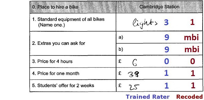
This function needs three data frames: one containing the data to be
aggregated (dat), one containing the subunit information
(subunits), and one containing the unit information
(units).
| vc | valid code |
| colnames | missing types to be aggregated |
| rownames | missing types to be aggregated |
Optionally, you can specify how missing values should be aggregated
(aggregatemissings) like in the example, or which column
names the returned data frame should have (recodedData),
for instance. Type ?aggregateData into your console to
learn more.
am <- matrix(c(
"vc" , "mvi", "vc" , "mci", "err", "vc" , "mbi", "err",
"mvi", "mvi", "err", "mci", "err", "err", "err", "err",
"vc" , "err", "mnr", "mci", "err", "mir", "mnr", "err",
"mci", "mci", "mci", "mci", "err", "mci", "mci", "err",
"err", "err", "err", "err", "mbd", "err", "err", "err",
"vc" , "err", "mir", "mci", "err", "mir", "mir", "err",
"mbi", "err", "mnr", "mci", "err", "mir", "mbi", "err",
"err", "err", "err", "err", "err", "err", "err", "err" ),
nrow = 8, ncol = 8, byrow = TRUE)
dimnames(am) <-
list(c("vc" ,"mvi", "mnr", "mci", "mbd", "mir", "mbi", "err"),
c("vc" ,"mvi", "mnr", "mci", "mbd", "mir", "mbi", "err"))
# using datRec from the chapter "recodeData()"
datAggr <- aggregateData(datRec, inputList$subunits, inputList$units,
aggregatemissings = am, rename = TRUE, recodedData = TRUE,
suppressErr = TRUE, recodeErr = "mci", verbose = TRUE)
#> All aggregation rules will be defaulted to 'SUM', because no other type is currently supported.
#> Found 20 unit(s) with only one subunit in 'dat'. This/these subunit(s) will not be aggregated and renamed to their respective unit name(s).
#> 1 units were aggregated: I12.Scoring Data
The next step is to score a data set with special consideration of
missing values. The function scoreData() is very similar to
recodeData(), but with a few defaults that are better
suited for scoring. scoreData() will give warnings when
incomplete scoring information is found. Values without scoring
information will not be scored.
Again, you need to specify three data frames. One data frame that you
get after completing the steps you did so far or by using
automateDataPreparation (dat), one with
information about the scoring of units (unitrecodings), and
one with subunit information (subunits). Examples for the
last two data frames can be found via inputList.
prepDat <- automateDataPreparation (inputList = inputList, datList = inputDat,
readSpss = FALSE, checkData=FALSE, mergeData = TRUE, recodeData=TRUE,
aggregateData=TRUE, scoreData= FALSE, writeSpss=FALSE, verbose = TRUE)
datSco <- scoreData(prepDat, inputList$unitRecodings, inputList$subunits,
verbose = TRUE)
#> ✔ 1 unit was scored: `I12`.mnrCoding
Then you can convert missing responses coded as “missing by
intention” (mbi) at the end of a block of items to “missing
not reached” (mnr) via mnrCoding(). The
function returns a data frame with “missing not reached” coded as
mnr. For each person with at least one mnr in
the returned data set the names of recoded variables are given as an
attribute to dat.
For that to work you need to specify the following arguments, as they don’t have any default settings:
| Argument | Explanation |
|---|---|
| dat | A data set. Missing by intention needs to be coded
mbi
|
| pid | Name or column number of the identifier (ID) variable in
dat
|
| rotation.id | A character vector of length 1 indicating the column name of the
test booklet identifier in dat
|
| blocks | A data frame containing the sequence of subunits in each block in
long format. The column names need to be subunit,
block, subunitBlockPosition
|
| booklets | A data frame containing the sequence of blocks in each booklet in
wide format. The column names need to be booklet,
block1, block2, block3, … |
| breaks | Number of blocks after which mbi shall be recoded to
mnr, e.g., c(1,2) to specify breaks after the
first and second block |
There are more arguments with default values which you can specify, but don’t have to.
nMbi, for instance, specifies the number of subunits at
the end of a block that need to be coded mbi. The default
is 2, i.e. if the last and second to last subitem in a block are coded
mbi, both subunits, as well as the preceding subunits coded
mbi, will be recoded to mnr. If
nMbi is larger than the number of subunits in a given
block, no subitem in this block will be recoded. If all subunits in a
block are coded mbi, none of them will be recoded to
mnr. nMbi needs to be > 0.
subunits has the default NULL, but when you
specify a data frame, mnrCoding() expects to find the
recoded subunits in dat.
Examples for the data frames booklets,
blocks, rotation and subunits can
be found via inputList. Here is an example use case of
mnrCoding(). The first two functions
(automateDataPreparation() and mergeData())
create the data frame dat for mnrCoding().
prepDat <- automateDataPreparation(inputList = inputList,
datList = inputDat, readSpss = FALSE, checkData=FALSE,
mergeData = TRUE, recodeData=TRUE, aggregateData=FALSE,
scoreData= FALSE, writeSpss=FALSE, verbose = TRUE)
prepDat2 <- mergeData("ID", list(prepDat, inputList$rotation))
mnrDat <- mnrCoding(dat = prepDat2, pid = "ID",
booklets = inputList$booklets, blocks = inputList$blocks,
rotation.id = "booklet", breaks = c(1, 2),
subunits = inputList$subunits, nMbi = 2, mbiCode = "mbi",
mnrCode = "mnr", invalidCodes = c("mbd", "mir", "mci"),
verbose = TRUE)
#> ...identifying items in data (reference is blocks$subunit)
#> Variables in data not recognized as items:
#> ID, hisei, booklet
#> If some of these excluded variables should have been identified as items (and thus be used for mnr coding) check 'blocks', 'subunits', 'dat'.
#> ...identifying items with no mbi-codes ('mbi'):
#> I04R, I08R
#> If you expect mbi-codes on these variables check your data and option 'mbiCode'
#> mnr statistics:
#> mnr cells: 553
#> unique cases with at least one mnr code: 89
#> unique items with at least one mnr code: 16
#> unique cases ('ID') per booklet and booklet section (0s omitted):
#> booklet booklet.section N.ID
#> 1 booklet1 2 11
#> 2 booklet1 3 28
#> 3 booklet2 1 28
#> 4 booklet2 2 11
#> 5 booklet2 3 1
#> 6 booklet3 3 31
#> start recoding (item-wise)
#> done
#> elapsed time: 0.0 secsType ?mnrCoding into your console to learn more.
Wrapper
Instead of using all the individual functions as described above, you
can also use the wrapper function automateDataPreparation,
which contains most of the described functions. Here is an overview over
the arguments that call the corresponding function.
| Argument | Corresponding Function |
|---|---|
readSpss |
readSpss() |
checkData |
checkData() |
mergeData |
mergeData() |
recodeData |
recodeData() |
recodeMnr |
mnrCoding() |
aggregateData |
aggregateData() |
scoreData |
scoreData() |
collapseMissings |
collapseMissings() |
writeSpss |
writeSpss() |
But there are many more arguments that may need to be considered. For
more information see ?automateDataPreparation.
Here is an example use case and its output.
automateDataPreparation returns a data frame resulting from
the final data preparation step.
data(inputList)
data(inputDat)
preparedData <- automateDataPreparation(inputList = inputList,
datList = inputDat, path = getwd(),
readSpss = FALSE, checkData = TRUE, mergeData = TRUE,
recodeData = TRUE, recodeMnr = TRUE, breaks = c(1,2),
aggregateData = TRUE, scoreData = TRUE,
writeSpss = FALSE, verbose = TRUE)
#> Starting automateDataPreparation 2026-10-17 09:44:57.411259
#>
#> Check data...
#>
#> Checking dataset booklet1
#> Only valid codes in ID variable.
#> No duplicated entries in ID variable.
#> No duplicated variable names.
#> Found no variable information about variable(s) hisei. This/These variables will not be checked for missings and invalid codes.
#> Found no invalid codes.
#>
#> Checking dataset booklet2
#> Only valid codes in ID variable.
#> No duplicated entries in ID variable.
#> No duplicated variable names.
#> Found no variable information about variable(s) hisei. This/These variables will not be checked for missings and invalid codes.
#> Found no invalid codes.
#>
#> Checking dataset booklet3
#> Only valid codes in ID variable.
#> No duplicated entries in ID variable.
#> No duplicated variable names.
#> Found no variable information about variable(s) hisei. This/These variables will not be checked for missings and invalid codes.
#> Found no invalid codes.
#>
#> Start merging.
#> Start merging of dataset 1.
#> Start merging of dataset 2.
#> Start merging of dataset 3.
#> Start adding mbd according to data pattern.
#>
#> Start recoding.
#>
#> Found no recode information for variable(s):
#> ID, hisei.
#> This/These variable(s) will not be recoded.
#>
#> Variables... I01, I02, I03, I04, I05, I06, I07, I08, I09, I10, I11, I12a, I12b, I12c, I13, I14, I15, I16, I17, I18, I19, I20, I21, I22, I23, I24, I25, I26, I27, I28
#> ...have been recoded.
#>
#> Start recoding Mbi to Mnr.
#> ...identifying items in data (reference is blocks$subunit)
#> Variables in data not recognized as items:
#> ID, booklet, hisei
#> If some of these excluded variables should have been identified as items (and thus be used for mnr coding) check 'blocks', 'subunits', 'dat'.
#> ...identifying items with no mbi-codes ('mbi'):
#> I04R, I08R
#> If you expect mbi-codes on these variables check your data and option 'mbiCode'
#> mnr statistics:
#> mnr cells: 553
#> unique cases with at least one mnr code: 89
#> unique items with at least one mnr code: 16
#> unique cases ('ID') per booklet and booklet section (0s omitted):
#> booklet booklet.section N.ID
#> 1 booklet1 2 11
#> 2 booklet1 3 28
#> 3 booklet2 1 28
#> 4 booklet2 2 11
#> 5 booklet2 3 1
#> 6 booklet3 3 31
#> start recoding (item-wise)
#> done
#> elapsed time: 0.0 secs
#>
#> Start aggregating
#> Since inputList$aggrMiss exists, this will be used instead of default.
#> All aggregation rules will be defaulted to 'SUM', because no other type is currently supported.
#> Found 27 unit(s) with only one subunit in 'dat'. This/these subunit(s) will not be aggregated and renamed to their respective unit name(s).
#> 1 units were aggregated: I12.
#>
#> Start scoring.
#> ✔ 1 unit was scored: `I12`.
#>
#> No SPSS-File has been written.
#>
#> Missings are UNcollapsed.
#> automateDataPreparation terminated successfully! 2026-10-17 09:44:57.560069Additional Diagnostics and Rater Tools
The functions above cover the main data preparation pipeline.
eatPrep also contains tools for category diagnostics, rater
agreement, IDM cut scores and semi-manual recoding of flagged
subsets.
Category Discrimination
catPbc() calculates category-level point-biserial
correlations. It compares a merged raw data set with the corresponding
recoded data set and returns frequencies and correlations for each item
category. This is useful for finding recoding mistakes or suspicious
item categories before scaling.
datRaw <- mergeData(newID = "ID", datList = inputDat, addMbd = TRUE)
#> Start merging of dataset 1.
#> Start merging of dataset 2.
#> Start merging of dataset 3.
#> Start adding mbd according to data pattern.
datRecPbc <- recodeData(datRaw, values = inputList$values,
subunits = inputList$subunits, verbose = FALSE)
pbcs <- catPbc(datRaw, datRecPbc, idRaw = "ID", idRec = "ID",
context.vars = "hisei", values = inputList$values,
subunits = inputList$subunits)
head(pbcs)
#> item cat n freq freq.rel catPbc recodevalue subunitType
#> 1 I01 1 200 27 0.135 -0.05898175 0 1
#> 2 I01 2 200 84 0.420 -0.35201750 0 1
#> 3 I01 3 200 35 0.175 0.15887365 1 1
#> 4 I01 8 200 48 0.240 0.26930074 mir 1
#> 5 I01 9 200 6 0.030 0.10854342 mbi 1
#> 6 I02 1 200 19 0.095 0.13417790 1 1evalPbc() evaluates the output of catPbc()
against configurable thresholds. It returns an empty list if no
problematic categories are found; otherwise it returns item names
grouped by the type of potential problem.
evalPbc(pbcs)
#> ✖ The attractors (score 1) of the following 1 item were chosen with a frequency
#> of zero: I14. This should not happen. Please check.
#> ! The distractors (score 0) of the following 1 item were chosen with a
#> frequency of zero: I14_7. This may happen, but is probably not intended.
#> ✖ catPbcs for attractors (score 1) of the following 3 items are worrisome low (< 0.05) or missing: I12c:_0.01, I14:_NA, and I24:_-0.12
#> ✖ catPbcs for distractors (score 0) of the following 9 items are unexpectedly high (> 0.005): I02_4_0.11, I07_3_0.26, I07_4_0.03, I12c_3_0.03, I13_4_0.01, I14_4_0.06, I14_5_0.04, I15_3_0.03, I17_1_0.06, I17_3_0.04, I22_3_0.13, and I24_1_0.21
#> ! catPbcs for mistype 'mir' of the following 3 items are relatively high (>
#> 0.07): I01_8_0.27, I03_8_0.29, and I16_8_0.08
#> ! catPbcs for mistype 'mbi' of the following 8 items are relatively high (>
#> 0.07): I01_9_0.11, I02_9_0.15, I16_9_0.14, I17_9_0.16, I18_9_0.19, I20_9_0.14,
#> I21_9_0.15, and I23_9_0.17
#> ℹ For a list of problematic items, save the `output` of this function and
#> return the item names as a vector:
#> • `output$zeroFreqAtt`
#> • `output$zeroFreqDis`
#> • `output$lowMisPbcAtt`
#> • `output$highPbcDis`
#> • `output$highPbcMis$mir`
#> • `output$highPbcMis$mbi`Rater Agreement
meanAgree() and meanKappa() summarize
pairwise agreement between several raters. The input is a wide data
frame with persons in rows and raters in columns. If your rater data are
in long format, you can reshape them first.
Pseudo Raters
make.pseudo() reduces ratings from multiple real raters
to a smaller number of pseudo raters. This is useful when later
processing steps require a fixed number of ratings per response.
Optional arguments such as alwaysPrefer,
alwaysNeglect and item.groups let you control
which raters should be preferred and whether linked variables should
stay with the same pseudo rater where possible.
oneRater <- make.pseudo(datLong = rater, idCol = "id", varCol = "variable",
codCol = "rater", valueCol = "value", n.pseudo = 1,
verbose = TRUE)
#> N.persons: 1287
#> N.vars: 7
#> N.coder: 4
#> coders per response: minimum 2, maximum 2
#> responses with multiple ratings: 2100 of 2100 (100 %)
head(oneRater)
#> id rater variable value index
#> P0002 P0002 John V01 1 P0002_V01
#> P0009 P0009 Carol V01 0 P0009_V01
#> P0010 P0010 Edward V01 0 P0010_V01
#> P0020 P0020 John V01 9 P0020_V01
#> P0022 P0022 Carol V01 1 P0022_V01
#> P0024 P0024 Dolores V01 0 P0024_V01IDM Cut Scores
computeCutsIDM() calculates cut scores for Item
Descriptor Matching (IDM). The preferred input is a long-format data set
with item identifiers, item difficulty estimates, a rater identifier,
and one rating column. Rater identifiers may be names or IDs. Ratings
may be numeric, or they may be ordinal labels when their order is
supplied via rating_levels. The previous wide-format input
with one rating column per rater is still supported.
idmDat <- data.frame(
item = rep(paste0("item_", 1:8), 3),
est = rep(seq(-2, 2, length.out = 8), 3),
rater = rep(c("Meyer", "Schmidt", "Tran"), each = 8),
rating = c(
"1a", "1a", "1b", "2", "2", "3", "4", "4",
"1a", "1b", "1b", "2", "3", "3", "4", "4",
"1a", "1a", "1b", "1b", "2", "3", "3", "4"
)
)
cuts <- computeCutsIDM(
idmDat,
item_id_col = "item",
rater_id_col = "rater",
rating_col = "rating",
rating_levels = c("1a", "1b", "2", "3", "4")
)
cuts$cuts_summary
#> # A tibble: 1 × 4
#> cut_1a_1b cut_1b_2 cut_2_3 cut_3_4
#> <dbl> <dbl> <dbl> <dbl>
#> 1 -1.38 -0.429 0.429 1.38
cuts$cut_statistics
#> # A tibble: 3 × 9
#> statistic page_cut_1a_1b page_cut_1b_2 page_cut_2_3 page_cut_3_4
#> <chr> <dbl> <dbl> <dbl> <dbl>
#> 1 Mean 2.08 3.75 5.25 6.92
#> 2 SD 0.520 0.5 0.5 0.520
#> 3 SE 0.300 0.289 0.289 0.300
#> # ℹ 4 more variables: diff_cut_1a_1b <dbl>, diff_cut_1b_2 <dbl>,
#> # diff_cut_2_3 <dbl>, diff_cut_3_4 <dbl>
cuts$level_statistics
#> # A tibble: 5 × 5
#> level interval n_items mean_itemdiff sd_itemdiff
#> <int> <chr> <int> <dbl> <dbl>
#> 1 1 [-2,-1.38) 2 -1.71e+ 0 0.404
#> 2 2 [-1.38,-0.43) 1 -8.57e- 1 NA
#> 3 3 [-0.43,0.43) 2 -1.11e-16 0.404
#> 4 4 [0.43,1.38) 1 8.57e- 1 NA
#> 5 5 [1.38,2] 2 1.71e+ 0 0.404
cuts$modal_values
#> # A tibble: 8 × 11
#> item_position item_id est n_ratings modal_n modal_prop modal_stage
#> <int> <chr> <dbl> <int> <int> <dbl> <dbl>
#> 1 1 item_1 -2 3 3 1 1
#> 2 2 item_2 -1.43 3 2 0.667 1
#> 3 3 item_3 -0.857 3 3 1 2
#> 4 4 item_4 -0.286 3 2 0.667 3
#> 5 5 item_5 0.286 3 2 0.667 3
#> 6 6 item_6 0.857 3 3 1 4
#> 7 7 item_7 1.43 3 2 0.667 5
#> 8 8 item_8 2 3 3 1 5
#> # ℹ 4 more variables: modal_label <chr>, modal_stages <chr>,
#> # modal_labels <chr>, tie <lgl>
cuts$rater_modal_correlations
#> # A tibble: 3 × 5
#> person n_items_modal_all cor_modal_all n_items_modal_loo
#> <chr> <int> <dbl> <int>
#> 1 Meyer 8 1 4
#> 2 Schmidt 8 0.958 6
#> 3 Tran 8 0.958 6
#> # ℹ 1 more variable: cor_modal_leave_one_out <dbl>
cuts$rater_kappa_statistics
#> # A tibble: 3 × 5
#> person n_pairs mean_kappa sd_kappa mean_n_items
#> <chr> <int> <dbl> <dbl> <dbl>
#> 1 Meyer 2 0.692 0 8
#> 2 Schmidt 2 0.532 0.226 8
#> 3 Tran 2 0.532 0.226 8
cuts$fleiss_kappa
#> # A tibble: 1 × 6
#> method n_items n_raters kappa statistic p_value
#> <chr> <int> <int> <dbl> <dbl> <dbl>
#> 1 Fleiss 8 3 0.583 5.69 0.0000000125
cuts$icc_statistics
#> # A tibble: 2 × 14
#> type model unit n_items n_raters icc_name icc f_value df1 df2 p_value
#> <chr> <chr> <chr> <int> <int> <chr> <dbl> <dbl> <dbl> <dbl> <dbl>
#> 1 agree… twow… sing… 8 3 ICC(A,1) 0.93 56.8 7 14 3.30e-9
#> 2 consi… twow… sing… 8 3 ICC(C,1) 0.949 56.8 7 14 3.30e-9
#> # ℹ 3 more variables: conf_level <dbl>, lbound <dbl>, ubound <dbl>
summary(cuts)
#> IDM cut-score summary
#>
#> Settings
#> input_format missing est_col item_id_col n_raters n_items n_cuts
#> long drop est item 3 8 4
#>
#> Boundaries
#> cut boundary lower_level upper_level
#> cut_1a_1b 1.5 1a 1b
#> cut_1b_2 2.5 1b 2
#> cut_2_3 3.5 2 3
#> cut_3_4 4.5 3 4
#>
#> Mean cuts on difficulty scale
#> cut_1a_1b cut_1b_2 cut_2_3 cut_3_4
#> -1.38 -0.43 0.43 1.38
#>
#> Cut statistics
#> statistic page_cut_1a_1b page_cut_1b_2 page_cut_2_3 page_cut_3_4
#> Mean 2.08 3.75 5.25 6.92
#> SD 0.52 0.50 0.50 0.52
#> SE 0.30 0.29 0.29 0.30
#> diff_cut_1a_1b diff_cut_1b_2 diff_cut_2_3 diff_cut_3_4
#> -1.38 -0.43 0.43 1.38
#> 0.30 0.29 0.29 0.30
#> 0.17 0.16 0.16 0.17
#>
#> Level statistics
#> level interval n_items mean_itemdiff sd_itemdiff
#> 1 [-2,-1.38) 2 -1.71 0.4
#> 2 [-1.38,-0.43) 1 -0.86 NA
#> 3 [-0.43,0.43) 2 0.00 0.4
#> 4 [0.43,1.38) 1 0.86 NA
#> 5 [1.38,2] 2 1.71 0.4
#>
#> Modal values per item
#> item_position item_id est n_ratings modal_n modal_prop modal_stage
#> 1 item_1 -2.00 3 3 1.00 1
#> 2 item_2 -1.43 3 2 0.67 1
#> 3 item_3 -0.86 3 3 1.00 2
#> 4 item_4 -0.29 3 2 0.67 3
#> 5 item_5 0.29 3 2 0.67 3
#> 6 item_6 0.86 3 3 1.00 4
#> 7 item_7 1.43 3 2 0.67 5
#> 8 item_8 2.00 3 3 1.00 5
#> modal_label modal_stages modal_labels tie
#> 1a 1 1a FALSE
#> 1a 1 1a FALSE
#> 1b 2 1b FALSE
#> 2 3 2 FALSE
#> 2 3 2 FALSE
#> 3 4 3 FALSE
#> 4 5 4 FALSE
#> 4 5 4 FALSE
#>
#> Rater correlations with modal values
#> person n_items_modal_all cor_modal_all n_items_modal_loo
#> Meyer 8 1.00 4
#> Schmidt 8 0.96 6
#> Tran 8 0.96 6
#> cor_modal_leave_one_out
#> 1.00
#> 0.95
#> 0.95
#>
#> Pairwise Cohen kappa summary
#> n_pairs mean_kappa sd_kappa mean_n_items
#> 3 0.59 0.18 8
#>
#> Rater pairwise Cohen kappa
#> person n_pairs mean_kappa sd_kappa mean_n_items
#> Meyer 2 0.69 0.00 8
#> Schmidt 2 0.53 0.23 8
#> Tran 2 0.53 0.23 8
#>
#> Fleiss kappa
#> method n_items n_raters kappa statistic p_value
#> Fleiss 8 3 0.58 5.69 0
#>
#> ICC agreement and consistency
#> type model unit n_items n_raters icc_name icc f_value df1 df2
#> agreement twoway single 8 3 ICC(A,1) 0.93 56.8 7 14
#> consistency twoway single 8 3 ICC(C,1) 0.95 56.8 7 14
#> p_value conf_level lbound ubound
#> 0 0.95 0.76 0.98
#> 0 0.95 0.84 0.99When rating_levels is supplied, ratings are mapped to
stage scores 1, 2, …, K in the
specified order; otherwise numeric ratings are used unchanged. For each
rater, items are ordered by difficulty, retaining their first input
order for ties. The raw stage sequence is smoothed by a centered
three-point moving average. Its lower padding value is the minimum of
all observed stages across raters and
floor(min(boundaries)); its upper padding value is the
maximum of all observed stages and
ceiling(max(boundaries)). Sequences with fewer than three
entries are left unsmoothed. The smoothed sequence is then monotonized
with equally weighted isotonic regression, because IDM assumes that
expected rating stages should not decrease as item difficulty increases.
Tied difficulties receive the same fitted value.
By default, missing ratings are removed before smoothing the
remaining sequence, so neighboring available ratings can span missing
items; missing rows stay missing in the output series. In long-format
input, omitted item-rater rows are completed internally and treated like
explicit missing ratings. Use item_id_col whenever item
identities should be preserved explicitly, especially when different
items can have the same difficulty estimate. With
missing = "smooth", windows retain their original item
positions and ignore missing entries, potentially producing smoothed
values at missing ratings; an empty window remains missing. With this
option, the short-sequence rule counts all items, whereas the default
counts available ratings. Use missing = "error" to reject
incomplete ratings. The boundaries argument determines the
requested cut scores. Canonical boundaries such as 1.5 and
2.5 describe cuts between adjacent levels; non-canonical
boundaries are included in the generated cut labels.
Cut scores are interpolated boundary crossings of the monotonized
curves. For example, the default boundary 2.5 is the
transition between the second and third ordinal stage, here labelled
cut_1b_2. A boundary at or below the first fitted value
uses the first retained item; an unreached boundary yields
NA. With fewer than two finite smoothed values, all cuts
for that rater are NA. cuts_per_person reports
cuts on the item difficulty scale, and cuts_summary
averages the available rater-specific cuts separately for each boundary.
cut_positions_per_person stores interpolated positions in
the full ordered item list, while cut_statistics and
level_statistics summarize cuts and item difficulty
intervals. See the function reference
for the formulas and edge cases.
Additional agreement diagnostics are computed on the raw internal
rating stages, after long- and wide-format input have been normalized to
the same complete item-by-rater grid. modal_values gives
the item-wise modal rating stage. If the modal value is tied, the unique
modal_stage is set to NA, while
modal_stages, modal_labels, and
tie keep the tie information.
rater_modal_correlations correlates each individual rater
series with the modal-value series. The leave-one-rater-out version
recomputes the modal value without the currently evaluated rater, so the
rater is compared with the remaining group rather than with a criterion
partly defined by their own ratings.
The kappa diagnostics use the same wide raw rating matrix.
kappa_pairwise contains all pairwise Cohen kappa estimates
from meanKappa(). kappa_summary summarizes
these pairwise kappas overall, and rater_kappa_statistics
gives each rater’s mean and sample standard deviation across all
pairings involving that rater. Fleiss kappa and the two ICC estimates
for agreement and consistency are computed on complete item rows,
because these procedures require a common set of items across raters. If
the third, final IDM round is the target, filter the data to that round
before calling computeCutsIDM().
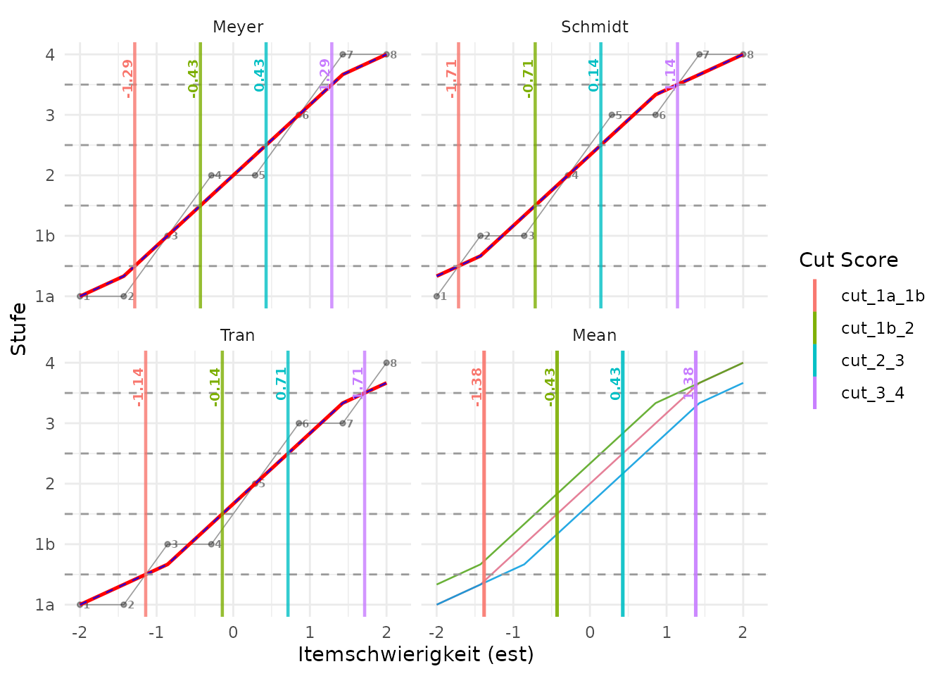
plotCutsIDM() visualizes the raw ratings, moving
averages, monotonized curves and resulting cut scores. Grey points and
lines show the original ratings ordered by item difficulty. The dashed
blue line shows the smoothed but not yet monotonized moving average. The
red line shows the monotonized curve used for the cut computation.
Because this example uses a compact item difficulty scale, the plot
examples show cut labels with two digits after the decimal point.
plotCutsIDM(cuts, cut_value_digits = 2)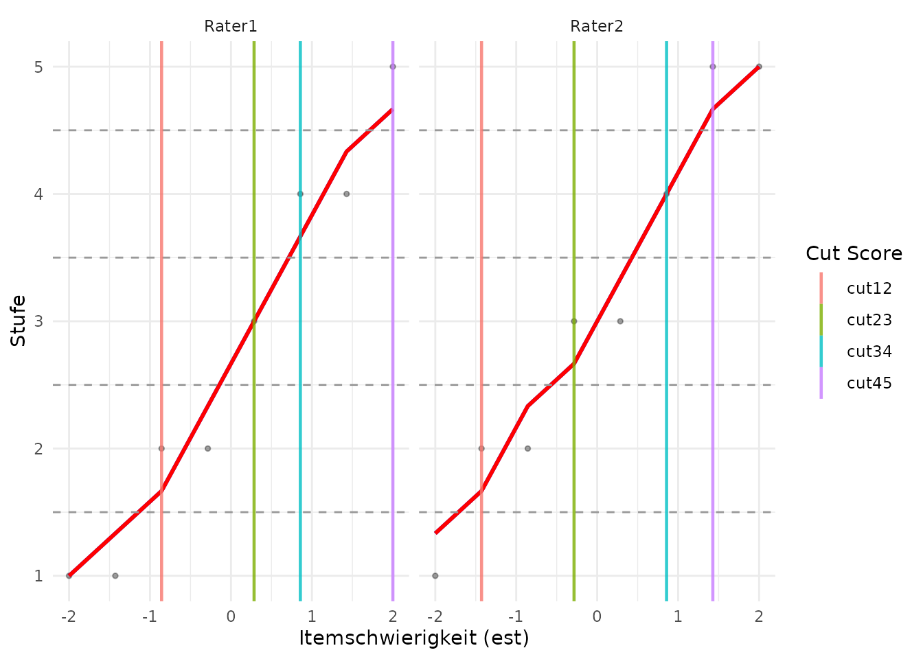
An aggregate panel can be added to inspect all monotonized rater
curves together with the mean cuts. In this panel, rater curves are
drawn in rater-specific colors and labelled by rater name by default.
When several curves end at similar values, the labels are shifted
slightly along the y-axis so that all names remain visible. The color
legend remains restricted to the cut score labels. The vertical cut
lines are the means from cuts$cuts_summary, not newly
estimated cuts from a pooled rating curve.
plotCutsIDM(cuts, show_aggregate = TRUE, cut_value_digits = 2)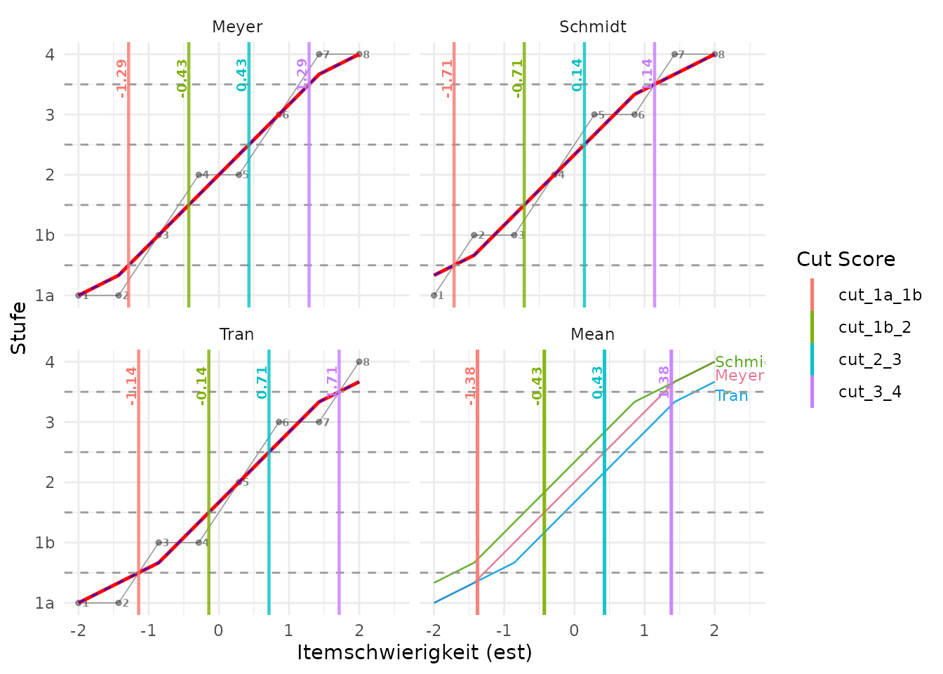
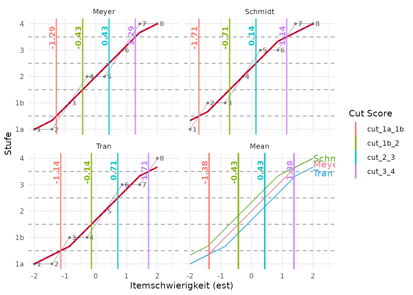
Adjust the text sizes inside the graph with
item_number_size (item positions),
cut_value_size (numeric cuts), and
aggregate_label_size (rater names in the aggregate panel).
Sizes are in millimetres, with defaults of 2,
2.6, and 3, respectively. These settings also
apply when residual panels are shown.
plotCutsIDM(
cuts,
show_aggregate = TRUE,
cut_value_digits = 2,
item_number_size = 3,
cut_value_size = 3.5,
aggregate_label_size = 4
)
Set show_aggregate_labels = FALSE if the direct labels
make the aggregate panel too dense.
plotCutsIDM(
cuts,
show_aggregate = TRUE,
show_aggregate_labels = FALSE,
cut_value_digits = 2
)
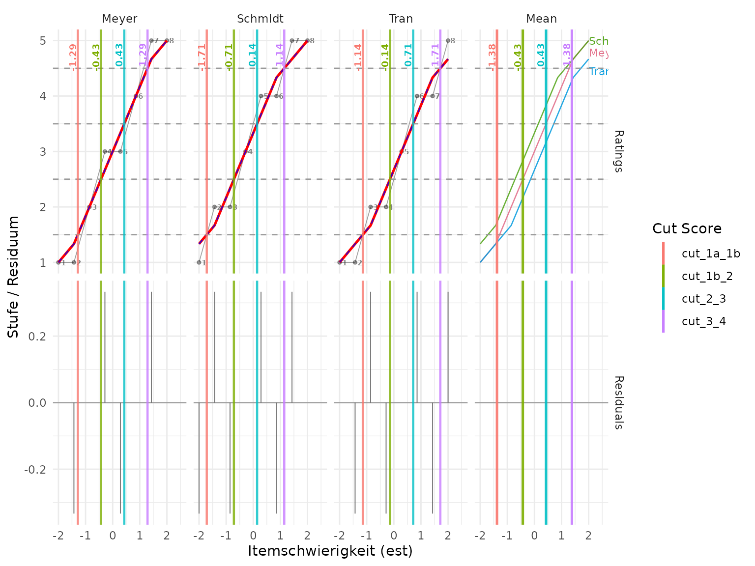
Residual panels can be added to inspect local deviations between raw ratings and the smoothed moving average. They can also be combined with the aggregate panel.
plotCutsIDM(
cuts,
show_residuals = TRUE,
show_aggregate = TRUE,
cut_value_digits = 2
)
Population Distributions and IDM Cuts
Population distributions from plausible values (PVs) can be displayed with estimated or supplied cuts:
| Purpose | Function | Meaning of the vertical axis |
|---|---|---|
| Inspect where the cuts divide the population distribution | plotPopulationCutsIDM() |
Population density |
| Use a numeric cut vector without an IDM result | plotPopulationCuts() |
Population density |
| Inspect the population alongside the rater curves | plotCutsIDM(..., pv_data = ...) |
Rating stages; the background silhouette shows distribution shape only |
The background silhouette’s height does not represent rating
stages or density-axis values. Its height is scaled for
display. Use the standalone population plot when you need a density
axis. Set show_caption = TRUE to include this explanation
below the plot; explanatory captions are hidden by default in both plot
functions.
Prepare population PVs on the cut-score metric
Pass a data frame for one domain, optionally with a
population_col identifying several populations. The PVs
must already be on the same metric as the item estimates and cuts: these
plotting functions do not transform scores or check that different
scales have been linked. Population respondents are distinct from the
raters and items used to calculate the cuts; no respondent-to-rater join
is performed.
The following synthetic data illustrate five PV columns and sampling
weights on the compact metric used by cuts above. In an
analysis, use the PVs and weights supplied with your population
data.
set.seed(42)
population <- data.frame(
student = seq_len(300),
weight = runif(300, 0.5, 2)
)
population_location <- rnorm(300, mean = 0, sd = 0.85)
pv_names <- paste0("PV", 1:5)
population[pv_names] <- replicate(
5, population_location + rnorm(300, sd = 0.3)
)
head(population)
#> student weight PV1 PV2 PV3 PV4 PV5
#> 1 1 1.8722091 -0.4257400 -0.5170118 0.03337537 -0.1559848 -0.01061738
#> 2 2 1.9056131 -1.3940874 -1.9037482 -1.19232003 -1.3625439 -1.78668443
#> 3 3 0.9292093 1.0433963 0.8898841 0.99354550 1.2079340 0.94064473
#> 4 4 1.7456714 -0.3536391 -0.1801812 -0.04690367 -0.3799261 -0.35818097
#> 5 5 1.4626183 -0.3662707 -1.0810018 -0.26832834 -0.2548810 -0.25028248
#> 6 6 1.2786439 -1.1481787 -0.9653571 -0.88502077 -0.8805684 -1.21188301Wide input has one row per respondent. Select PV columns explicitly
with pv_cols so that numeric IDs, weights, or PVs from
other domains cannot be included accidentally.
respondent_id_col is optional for wide input; when
supplied, its values must be unique. weight_col = NULL, the
default, gives every respondent equal weight. Supplied sampling weights
must be finite, non-missing and non-negative; zero-weight respondents
are excluded.
Density with supplied numeric cuts
Use plotPopulationCuts() when cut scores are already
available as a numeric vector. No IDM object is required. Cuts must be
finite and strictly increasing, and PVs must be on the same scale. For
example, these synthetic PVs use a score scale centered on 400:
score_population <- population
score_population[pv_names] <- lapply(population[pv_names], function(x) 400 + 100 * x)
supplied_cut_plot <- plotPopulationCuts(
cuts = c(230, 360, 460),
pv_data = score_population,
pv_cols = pv_names,
weight_col = "weight",
est_col = "points"
)
supplied_cut_plot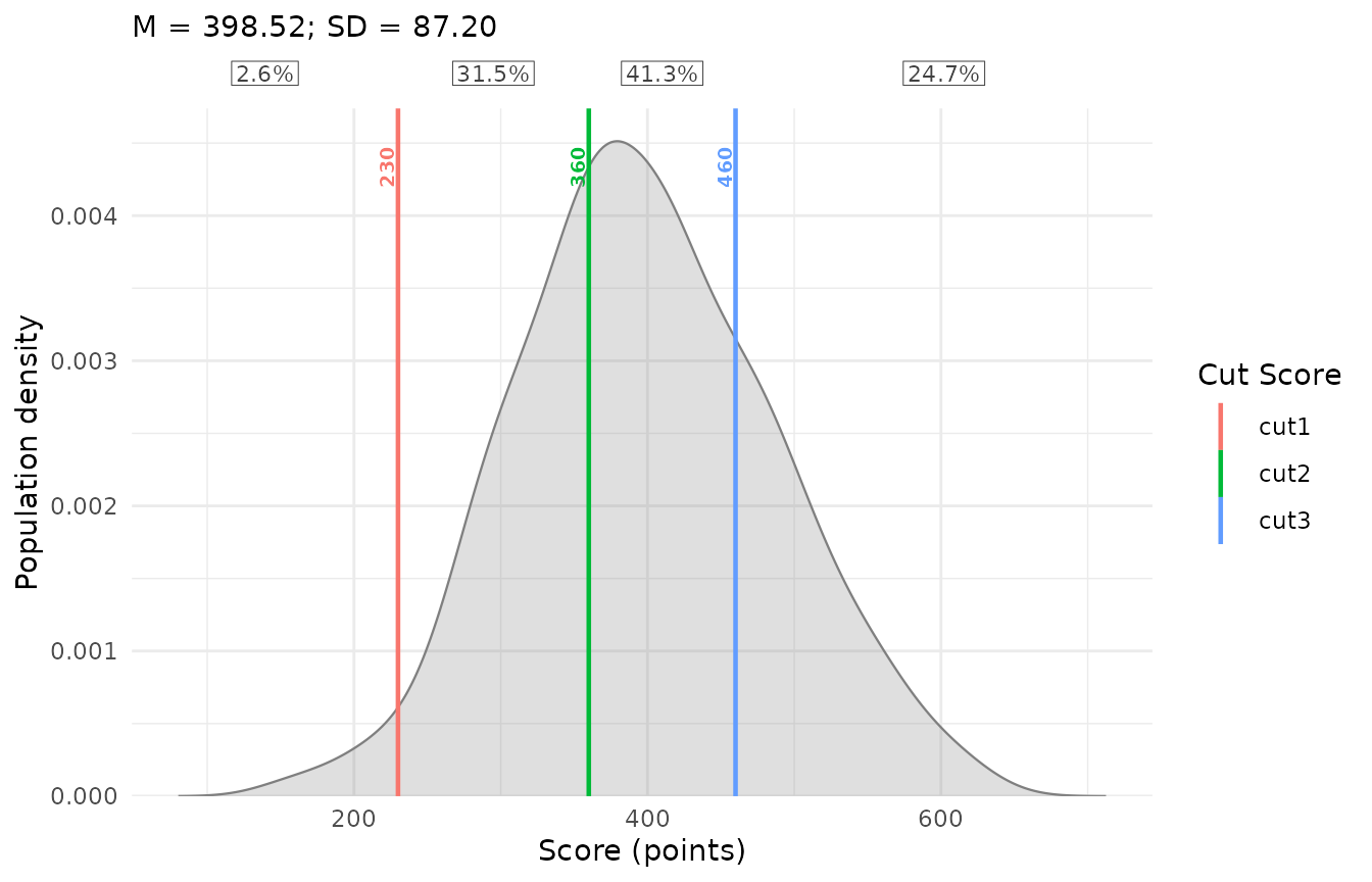
attr(supplied_cut_plot, "population_percentages")
#> population interval lower upper percentage
#> 1 Population 1 -Inf 230 2.602241
#> 2 Population 2 230 360 31.460002
#> 3 Population 3 360 460 41.280927
#> 4 Population 4 460 Inf 24.656831The returned attribute contains unrounded percentages and interval
bounds for each population. Values exactly on a cut enter the upper
interval. Percentages are computed separately per PV and then averaged;
density smoothing does not affect them.
show_percentages = FALSE hides the labels but retains this
table. The function also accepts the long-input selectors,
population_col, colors, and display options illustrated
below. cut_labels optionally names the cut lines in their
legend order.
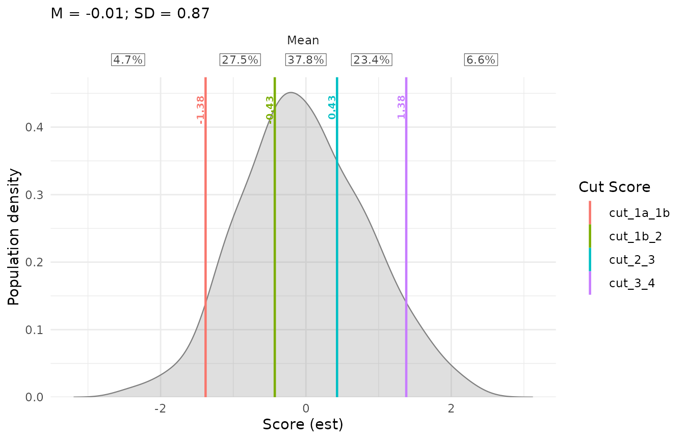
Standalone density with mean or individual cuts
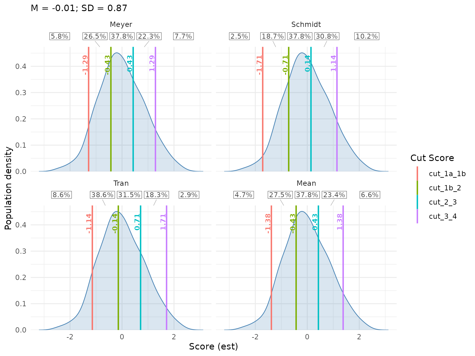
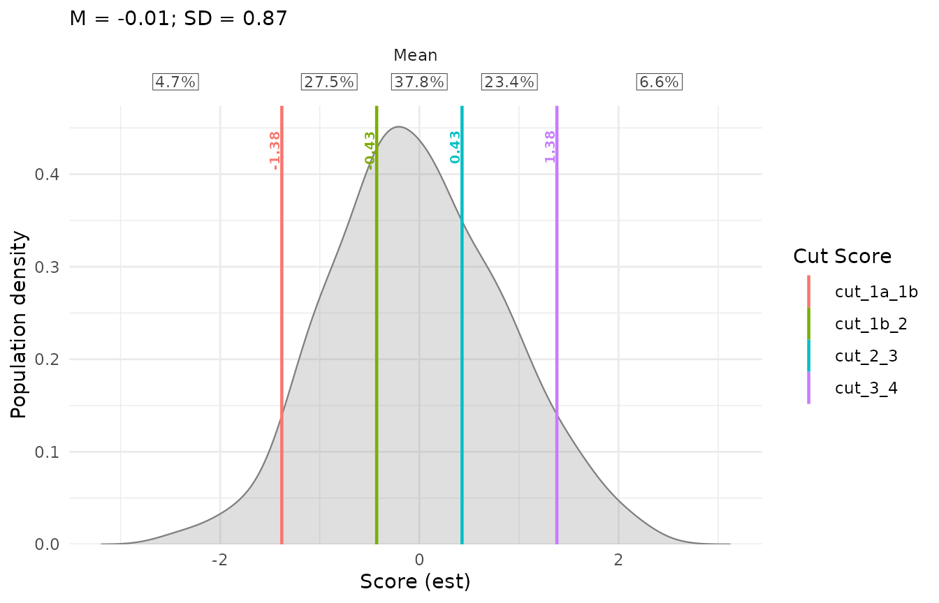
The default standalone plot draws the mean cuts from
cuts$cuts_summary over a lightly filled population density.
The vertical axis is density, and the cut lines use the supplied
difficulty-scale values without re-estimation.
plotPopulationCutsIDM(
cuts,
pv_data = population,
pv_cols = pv_names,
weight_col = "weight",
cut_value_digits = 2
)
Use cut_selection = "individual" for one facet per
rater, or "both" to include the mean-cut facet as well.
Every facet uses the same population distribution and fixed
axes; the distribution is not conditional on a rater. Use
population_fill and population_alpha for
appearance, and cut_value_size,
cut_value_digits, or show_cut_values = FALSE
for cut labels.
plotPopulationCutsIDM(
cuts,
pv_data = population,
pv_cols = pv_names,
weight_col = "weight",
cut_selection = "both",
cut_value_digits = 2,
cut_value_size = 3,
population_fill = "steelblue",
population_alpha = 0.2
)
Equivalent long-format input
Long input has one row per respondent and PV, with explicit
respondent ID, PV identifier, and numeric value columns. A respondent
must have the same sampling weight across all PV rows. Duplicate
respondent-PV rows cause an error. input_format = "auto"
selects long format when pv_id_col or
pv_value_col is supplied; explicit "wide" and
"long" are also supported.
population_long <- tidyr::pivot_longer(
population,
cols = dplyr::all_of(pv_names),
names_to = "pv",
values_to = "score"
)
# This gives the same distribution and mean cuts as the wide-input example.
plotPopulationCutsIDM(
cuts,
pv_data = population_long,
respondent_id_col = "student",
pv_id_col = "pv",
pv_value_col = "score",
weight_col = "weight",
cut_value_digits = 2
)
How PVs, weights, and smoothing are combined
Both functions estimate a Gaussian kernel density separately for each
PV, normalizing the available sampling weights to sum to one within each
PV. They then average the densities with equal weight across PVs on a
common grid with at least 512 points. The grid becomes finer when needed
to resolve narrow distributions or small bandwidths. If the requested
smoothing needs excessive grid resolution, increase
density_bw or density_adjust as indicated by
the error message. Do not average a respondent’s PVs
first: the distribution of respondent averages would discard
within-respondent PV variation. This follows the principle of computing
population estimates separately for each PV and averaging those
estimates, described in the OECD
PISA analysis guidance.
By default, the common bandwidth is the mean of
stats::bw.nrd0() bandwidths calculated separately for each
PV after exclusions. This avoids treating stacked PVs as additional
independently sampled respondents when selecting the bandwidth. The
automatic bandwidth rule is unweighted; sampling weights enter the
density calculation itself. Supply a positive density_bw in
score units to choose the bandwidth explicitly.
density_adjust multiplies that bandwidth: values above one
smooth more, and values below one smooth less. For example, add
density_adjust = 1.2 to either plotting call. The grid
extends three effective bandwidths beyond the observed PV range; all
finite plotted cuts are included in the displayed x-range.
These are descriptive population estimates. The plots do not compute uncertainty intervals or replicate-weight variances. Percentage tables are shown by default and are computed directly from PV observations, as explained below. A density height is not itself a percentage of respondents.
Missing values and incomplete long input
The default pv_missing = "error" rejects missing PV
values, including respondent-PV combinations omitted from long input.
With pv_missing = "drop", such values are omitted with a
warning, and weights are renormalized within each PV. Consequently,
different PVs can use different respondent subsets. Each PV must retain
at least two observed respondents with positive weights. Infinite PV
values and invalid or missing weights always cause an error.
population_incomplete <- population
population_incomplete$PV1[1] <- NA_real_
# Explicit omission produces a warning reporting the missing respondent-PV value.
population_plot_incomplete <- plotPopulationCutsIDM(
cuts,
pv_data = population_incomplete,
pv_cols = pv_names,
weight_col = "weight",
pv_missing = "drop"
)Include every intended PV identifier in long input. A PV that is entirely absent from the supplied data cannot be detected. The functions do not impute missing PVs.
Population silhouette behind rater curves
Supply pv_data to plotCutsIDM() to add the
population background. The PV input, weighting, and smoothing arguments
are identical to the standalone function. pv_data = NULL
preserves the existing plot.
Read the silhouette horizontally to locate the population
relative to the cuts. Its height communicates distribution shape only
and does not represent rating stages or density-axis values.
population_height = 0.25 places its peak at one quarter of
the rating range above the lower rating limit; this is a display choice,
not a statistical value. Changing population_height changes
neither the estimated density nor the cuts.
plotCutsIDM(
cuts,
show_aggregate = TRUE,
pv_data = population,
pv_cols = pv_names,
weight_col = "weight",
cut_value_digits = 2,
population_height = 0.25,
population_fill = "steelblue",
population_alpha = 0.15
)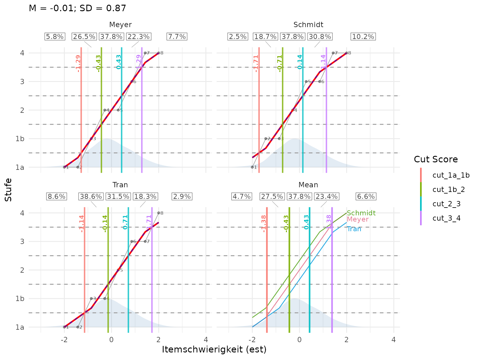
The population silhouette shows distribution shape only. Its height does not represent rating stages or density-axis values.
The same silhouette and height scaling are repeated in every rating
facet, including the aggregate panel. The rating axis, rater curves, cut
labels, and cut values keep their existing meaning. The shared x-range
expands to include the population distribution, so the item curves may
occupy a smaller part of the horizontal space. The explanatory plot
caption can be enabled with show_caption = TRUE.
Residual panels stay clear of the silhouette. The following example also demonstrates long-format input for the combined view.
plotCutsIDM(
cuts,
show_aggregate = TRUE,
show_residuals = TRUE,
pv_data = population_long,
respondent_id_col = "student",
pv_id_col = "pv",
pv_value_col = "score",
weight_col = "weight",
cut_value_digits = 2,
population_height = 0.25,
population_alpha = 0.15
)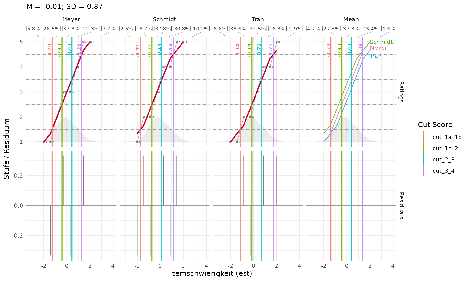
Only rating panels contain the population silhouette. Silhouette height shows distribution shape, not rating stages or density-axis values.
Compare two populations with overlapping distributions
Both functions accept population_col, the name of a
grouping column in the same wide or long PV data frame. Omitting it
preserves the single-population plots above. Group labels must be
non-missing and non-empty. Their order of first appearance determines
the drawing order and population legend; unused factor levels are
ignored.
Here we create a second synthetic population with fewer respondents, a higher location, and more dispersion. The student IDs deliberately repeat across populations. IDs must be unique within each population for wide input, and respondent-PV combinations must be unique within each population for long input. A respondent’s weight must be constant across PV rows within that population, but may differ between populations.
population_a <- transform(population, cohort = "Population A")
population_b <- transform(population[seq_len(220), ], cohort = "Population B")
population_b[pv_names] <- 1.35 * population_b[pv_names] + 0.7
populations <- rbind(population_a, population_b)
population_colors <- c(
"Population A" = "#0072B2",
"Population B" = "#E69F00"
)For each population, the functions average the densities estimated
from its own PVs and normalize weights within each PV. Each
population density has total area one. A larger sample or a
larger total sampling weight does not give that population a
proportionally larger curve. With pv_missing = "drop",
exclusions and weight renormalization occur separately within each
population and PV; diagnostic messages identify the affected population.
A PV entirely absent from a population’s long data cannot be
detected.
All populations share one bandwidth and one grid spanning their
combined observed PV range. The automatic bandwidth averages the per-PV
bandwidths within each population, then averages these population means
with equal weight. This also supports different numbers of PVs between
populations in long input. An explicit density_bw and
density_adjust apply to every population. Thus each
distribution can be compared under the same smoothing choice.
plotPopulationCutsIDM(
cuts,
pv_data = populations,
pv_cols = pv_names,
respondent_id_col = "student",
weight_col = "weight",
population_col = "cohort",
population_colors = population_colors,
population_alpha = 0.25,
cut_selection = "both",
cut_value_digits = 2
)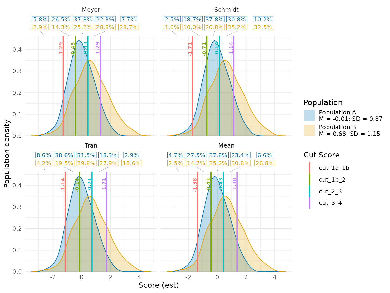
The filled densities overlap without stacking. Their outlines and a
separate Population legend identify the groups; the
Cut Score colors and legend keep their existing
meaning. Blue and orange are the defaults for two populations.
population_colors overrides these with a named color vector
containing exactly one entry for each observed population label. Reuse
that vector across figures for consistent colors. More than two groups
are supported, with a qualitative default palette.
Alternatively, set population_fill in either plot
function. An explicitly supplied single color, such as
population_fill = "grey50", colors all populations
alike. A vector with exactly one color per population follows
the order of first appearance in the data, which is also the legend
order; names on this vector are ignored. Grouped percentage rows, legend
keys, and density outlines follow the same colors. If you supply too
many or too few colors (except the single-color case), the plot warns
and uses its default palette. An empty vector also triggers this
fallback. Without grouping, the fallback is grey. Omitting
population_fill preserves the automatic colors; an
explicitly supplied population_colors takes precedence over
population_fill.
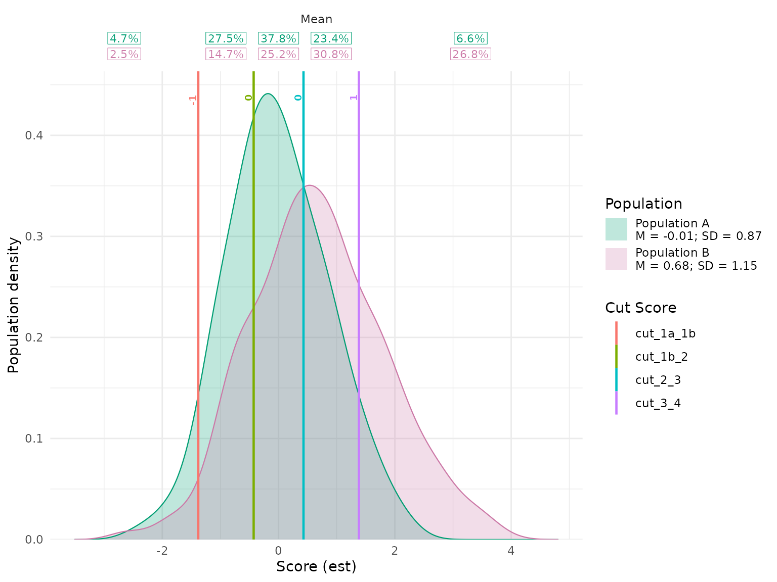
plotPopulationCutsIDM(
cuts, pv_data = populations, pv_cols = pv_names,
weight_col = "weight", population_col = "cohort",
population_fill = c("#009E73", "#CC79A7")
)
The same single color can be used for both populations in the rater background. Their names and statistics still appear separately in the legend. Silhouette height shows distribution shape only and does not represent rating stages.
plotCutsIDM(
cuts, pv_data = populations, pv_cols = pv_names,
weight_col = "weight", population_col = "cohort",
population_fill = "grey50"
)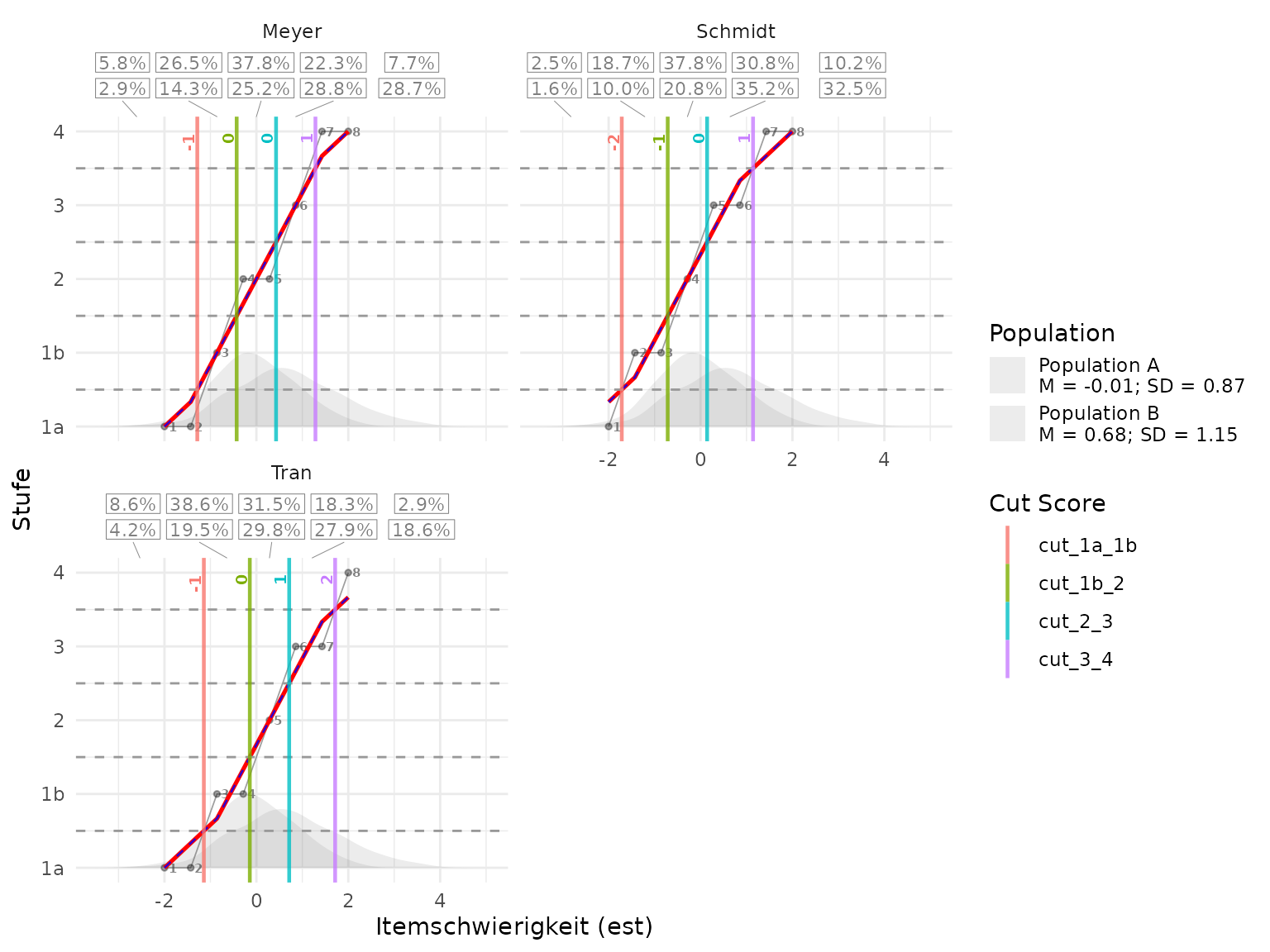
Both populations use the same color. Silhouette height shows distribution shape only and does not represent rating stages.
For these two populations,
population_fill = c("red", "blue", "green") would warn and
restore the default blue/orange palette.
For the rater background, all silhouettes use one shared
height factor. The highest density peak across all populations
occupies population_height times the rating range above its
lower limit. The other peaks retain their relative heights; the curves
are neither stacked nor individually stretched to the same peak. This
preserves visible differences in concentration.
The silhouettes still show distribution shape only. Their
shared display height does not represent rating stages or readable
density-axis values. Use plotPopulationCutsIDM()
when a density axis is needed. Use show_caption = TRUE to
include the silhouette explanation in the rater plot.
plotCutsIDM(
cuts,
pv_data = populations,
pv_cols = pv_names,
respondent_id_col = "student",
weight_col = "weight",
population_col = "cohort",
population_colors = population_colors,
population_height = 0.3,
population_alpha = 0.2,
show_aggregate = TRUE,
cut_value_digits = 2
)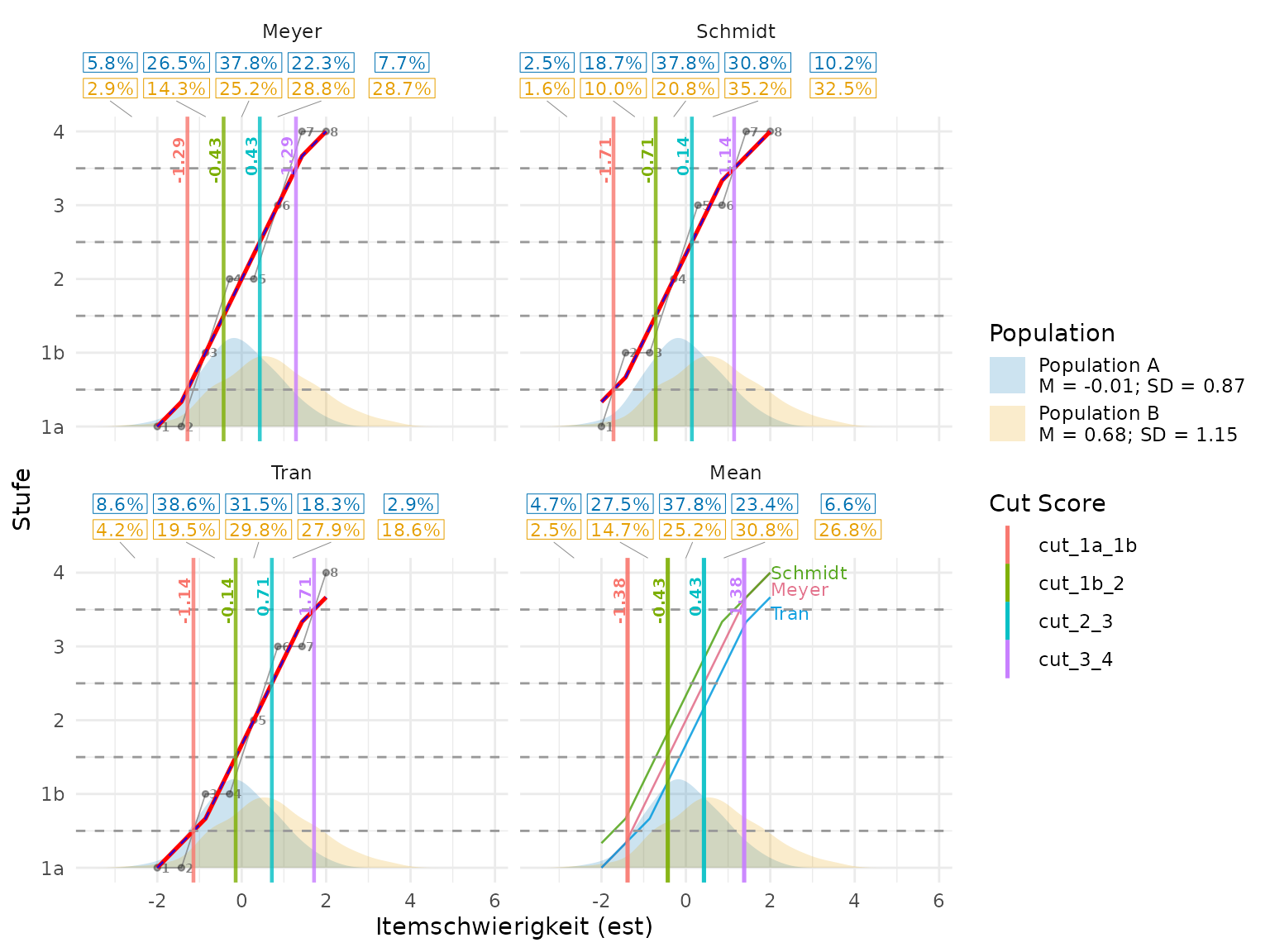
Both population silhouettes share a display-height factor. Their height shows distribution shape only, not rating stages or density-axis values.
All populations repeat in every rating and aggregate panel, while residual panels stay clear. The same grouped input can be supplied in long format to either function:
populations_long <- tidyr::pivot_longer(
populations, cols = dplyr::all_of(pv_names),
names_to = "pv", values_to = "score"
)
plotCutsIDM(
cuts,
pv_data = populations_long,
respondent_id_col = "student",
pv_id_col = "pv",
pv_value_col = "score",
weight_col = "weight",
population_col = "cohort",
population_colors = population_colors,
population_alpha = 0.2,
show_aggregate = TRUE,
show_residuals = TRUE,
cut_value_digits = 2
)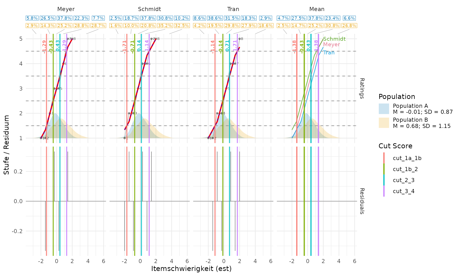
Population silhouettes appear only in rating panels. Their shared height scale communicates distribution shape and does not represent rating stages or density-axis values.
Population means and standard deviations
Both plotPopulationCutsIDM() and
plotCutsIDM() display M (mean) and
SD (standard deviation) below each population name in
the legend when PV data are supplied. With one ungrouped population,
these statistics appear in the subtitle. They use the supplied score
metric and describe the whole population, so one set of statistics
applies to all rater and mean-cut panels.
Means and variances are estimated separately for each PV and population using the supplied sampling weights. The final M is the average of the PV means; the final SD is the square root of the average PV variance. For \(m\) plausible values:
\[SD = \sqrt{\frac{1}{m}\sum_{j=1}^{m} SD_j^2}.\]
Every PV contributes equally. Respondents’ PVs are never averaged before estimating their population spread, and no variance component for differences between PV means is added.
Within a PV, the weighted mean squared deviation from that PV’s
weighted mean is multiplied by \(n_j/(n_j-1)\) before taking the square
root. Weights are normalized to sum to one, and \(n_j\) counts observed respondents with
positive weights in that PV and population after missing-data handling.
The correction is applied separately for every PV, so different numbers
of available respondents receive different correction factors. SD
describes population spread; it is not a standard error. For example,
with weights c(1, 3), PV1 values c(0, 4) have
M = 3 and corrected variance = 6, while PV2 values
c(18, 10) have M = 12 and corrected variance = 24. Here
each PV has two respondents, so each variance is multiplied by 2. The
displayed estimates are therefore M = 7.50 and SD = sqrt((6 + 24) / 2) =
3.87.
With pv_missing = "drop", each PV uses its available
observations and renormalized weights; zero-weight observations are
excluded. Changing cuts, zoom, or density smoothing does not change M or
SD. These estimates are calculated directly from the PV observations
before smoothing.
plotPopulationCutsIDM(
cuts,
pv_data = populations,
pv_cols = pv_names,
weight_col = "weight",
population_col = "cohort",
population_colors = population_colors,
cut_selection = "both",
population_stats_digits = 1,
show_caption = TRUE
)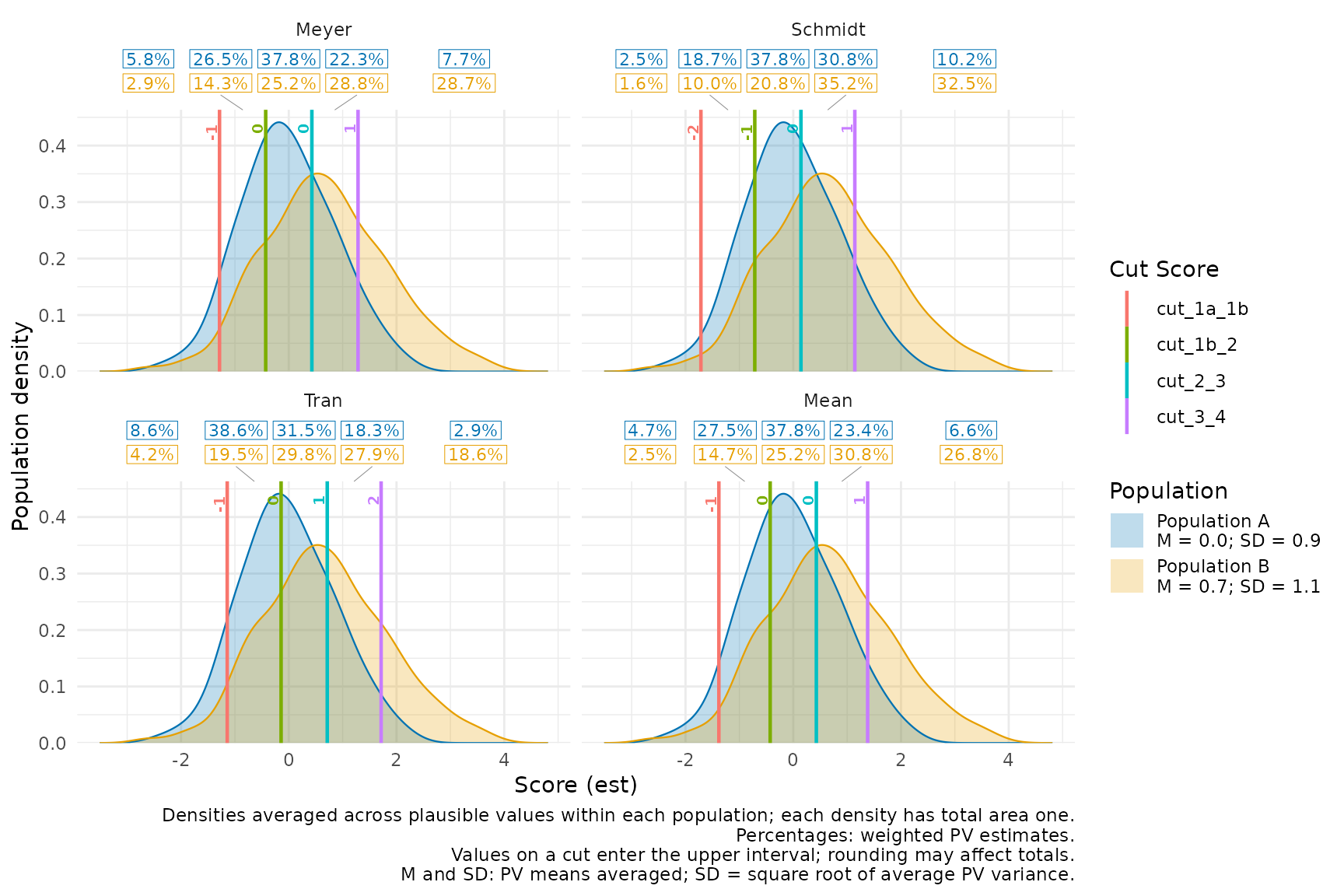
The same statistics are available with long-format population data in the rater view, including plots with residual panels:
plotCutsIDM(
cuts,
pv_data = populations_long,
respondent_id_col = "student",
pv_id_col = "pv",
pv_value_col = "score",
weight_col = "weight",
population_col = "cohort",
population_colors = population_colors,
show_aggregate = TRUE,
show_residuals = TRUE,
population_stats_digits = 1,
show_caption = TRUE
)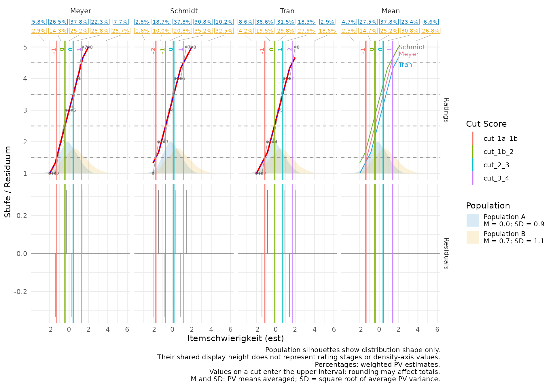
M and SD describe populations on the supplied score metric. Silhouette height communicates distribution shape only and does not represent rating stages.
Set show_population_stats = FALSE in either plot
function to hide M and SD. This is independent of
show_percentages, which controls the interval percentages.
population_stats_digits sets the decimal places (default
2); legend text size can be changed with
ggplot2::theme(legend.text = ggplot2::element_text(size = 10)),
or plot.subtitle for the ungrouped view. Explanatory
captions are hidden by default (show_caption = FALSE); the
two examples above explicitly enable them. This switch only controls
explanations below the plot and leaves M/SD in the legend or subtitle
and percentage labels unchanged. Without pv_data, the rater
plot is unchanged. Silhouette height in
plotCutsIDM() continues to communicate distribution shape
only and does not represent rating stages.
Population percentages within the cut intervals
Both plot functions now show population percentages by default when PV data are supplied. Each panel has a small table above its data, with a separate colored row for each population in legend order. Percentages follow the cut intervals from left to right. For one ungrouped population, the table has a single neutral row.
The percentage labels are estimated population shares.
Silhouette height still communicates distribution shape only and does
not represent rating stages or density-axis values. These
meanings are also explained in the optional plot captions
(show_caption = TRUE).
In general, there is one more interval than there are cuts. A value exactly on a cut belongs to the upper interval. The outer intervals extend to minus and plus infinity, so all available PV observations contribute, even when they fall outside a displayed x-axis window. The actual, unrounded cuts determine interval membership. Identical adjacent cuts create an empty interval with 0%; they are not merged.
Percentage labels are positioned midway between their visible cut boundaries. For the two outer intervals, they sit midway between the outermost cut and the corresponding visible panel edge. Both population rows use the same horizontal positions. When close or identical cuts would cause labels to overlap, the labels shift only as far as needed while preserving interval order. Thin connection lines point from shifted columns to their interval midpoints.
Placement uses the actual text widths when drawing, so it adapts to
resizing, zooming, and reversed score axes. Intervals wholly outside a
zoomed view are anchored at the nearest edge, while their estimated
shares still include all available PV observations. With many cuts or a
narrow plot, increase the figure width or reduce
percentage_size. If all labels together are wider than the
entire panel, text and padding are reduced together to keep them inside
it.
plotPopulationCutsIDM(
cuts,
pv_data = populations,
pv_cols = pv_names,
weight_col = "weight",
population_col = "cohort",
population_colors = population_colors,
cut_selection = "both",
cut_value_digits = 2,
show_percentages = TRUE,
percentage_digits = 1,
percentage_size = 3
)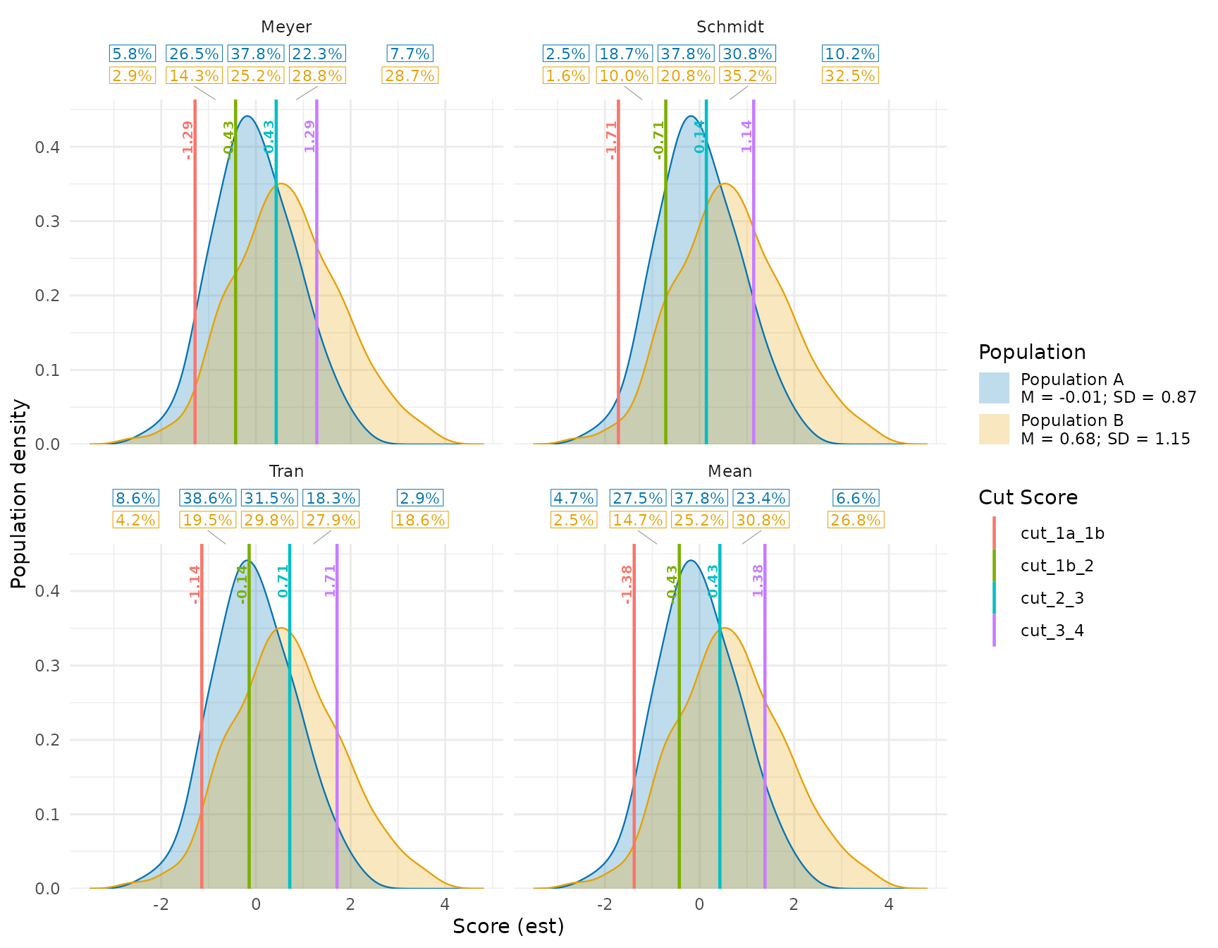
Each individual panel computes the shares using that rater’s cuts. The mean panel computes them using the mean cuts. Percentages at mean cuts are not averages of the raters’ percentages. The same panel cuts are applied separately to both populations so that their shares can be compared directly.
The following example deliberately uses unevenly spaced item
estimates, producing cuts that are close together. The short connection
lines identify intervals whose percentage labels need extra room. The
same positioning is used in plotCutsIDM().
uneven_items <- data.frame(
est = c(-2, -1.9, -1.8, -1.7, -1.6, -1.5, 0, 3),
Rater1 = c(1, 1, 2, 3, 4, 5, 5, 5)
)
uneven_cuts <- computeCutsIDM(uneven_items)
plotPopulationCutsIDM(
uneven_cuts,
pv_data = populations,
pv_cols = pv_names,
weight_col = "weight",
population_col = "cohort",
population_colors = population_colors,
cut_value_digits = 2
)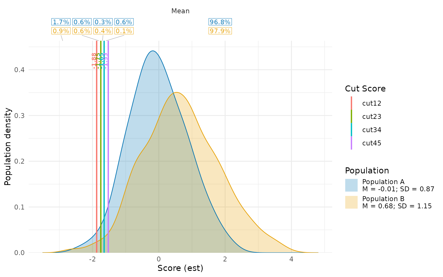
The calculation first obtains a weighted percentage within each PV:
the sum of weights in an interval divided by the total available weight,
multiplied by 100. It then averages those percentages equally across
PVs, separately for each population. Without weight_col,
this reduces to ordinary observed proportions within each PV.
Respondents’ PVs are never averaged before assigning values to
intervals.
For a hand-checkable illustration, suppose a panel has cuts at 0 and 10:
toy_pvs <- data.frame(
PV1 = c(-1, 0, 10, 11),
PV2 = c(1, -1, 9, 10),
weight = c(1, 2, 3, 4)
)
shares_at_0_and_10 <- function(x, w) {
100 * c(
sum(w[x < 0]),
sum(w[x >= 0 & x < 10]),
sum(w[x >= 10])
) / sum(w)
}
per_pv <- rbind(
PV1 = shares_at_0_and_10(toy_pvs$PV1, toy_pvs$weight),
PV2 = shares_at_0_and_10(toy_pvs$PV2, toy_pvs$weight)
)
colnames(per_pv) <- c("Below 0", "0 to below 10", "10 and above")
rbind(per_pv, Mean = colMeans(per_pv))
#> Below 0 0 to below 10 10 and above
#> PV1 10 20 70
#> PV2 20 40 40
#> Mean 15 30 55
# PV1: 10%, 20%, 70%; PV2: 20%, 40%, 40%; displayed estimate: 15%, 30%, 55%.With pv_missing = "drop", each population and PV uses
its own available observations and weight denominator after exclusions.
The previously documented checks for weights, IDs, and duplicate rows
still apply. Changing density_bw,
density_adjust, population_height, or
cut_value_digits cannot change percentage estimates: these
settings affect smoothing, silhouette display, or cut-label formatting,
not the underlying PV classifications.
The same percentage table is available in the combined rater view, including with long-format population data. It appears in rating and mean panels, never in residual panels:
plotCutsIDM(
cuts,
pv_data = populations_long,
respondent_id_col = "student",
pv_id_col = "pv",
pv_value_col = "score",
weight_col = "weight",
population_col = "cohort",
population_colors = population_colors,
show_aggregate = TRUE,
show_residuals = TRUE,
cut_value_digits = 2,
percentage_digits = 1,
percentage_size = 3
)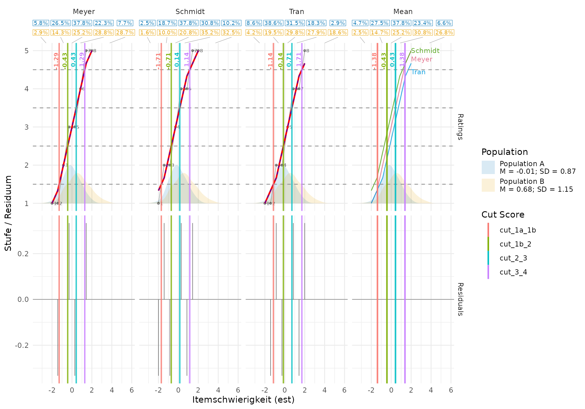
Numeric percentage labels estimate population shares. Silhouette height shows distribution shape only and does not represent rating stages or density-axis values.
percentage_digits controls displayed decimal places
(default 1, supported range 0 to 10); percentage_size
controls text size in millimetres (default 3). Tables reserve their own
space above each rating panel, so they remain clear of curves and cut
labels when the figure is resized. Increase figure height for many
raters or populations and figure width for many intervals. Percentages
are not adjusted to force rounded labels to total exactly 100%. Small
rounding differences are therefore possible. To hide the tables while
retaining distributions and numeric cut labels, set
show_percentages = FALSE in either function:
plotCutsIDM(
cuts,
pv_data = populations,
pv_cols = pv_names,
weight_col = "weight",
population_col = "cohort",
show_aggregate = TRUE,
cut_value_digits = 2,
show_percentages = FALSE
)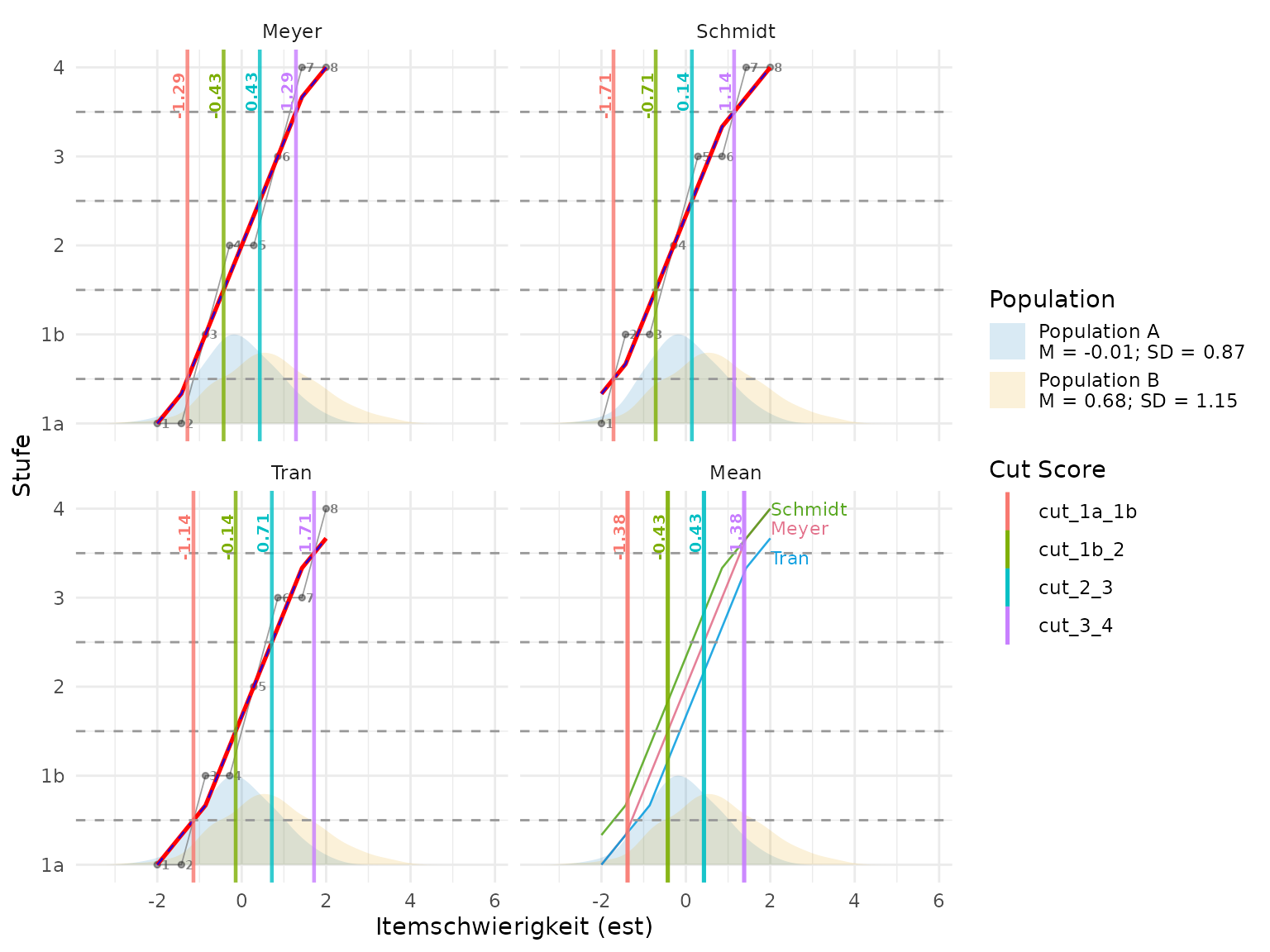
If a panel contains any missing or infinite cut, its percentage table is replaced with an explanatory message and a warning identifies the affected panel. Complete panels still show their percentages. Descending cut sequences cause an error when percentage computation is enabled. The estimates are descriptive point estimates; uncertainty intervals are not computed.
Logistic IDM Cut Scores
computeCutsIDMMAPT() provides a logistic comparison
using the same item difficulties and ratings. At each boundary it models
whether a rating is above that boundary, pooling the observed ratings.
Its cut is the difficulty where the fitted probability is 0.5. This is a
probability of a level assignment, not of a correct item response. The
calculation follows the regression step in the MAPT
Technical Manual (2006), pp. 54–55, without the report’s rating
trimming.
This example includes overlapping ratings so each logistic fit has information on both sides of the transition:
idmCompare <- data.frame(
item = paste0("I", 1:15),
est = seq(300, 650, length.out = 15),
Rater1 = c(1, 2, 1, 3, 2, 4, 3, 2, 5, 3, 4, 5, 4, 5, 4),
Rater2 = c(2, 1, 3, 1, 2, 3, 4, 3, 4, 5, 3, 4, 5, 4, 5)
)
cutsMA <- computeCutsIDM(idmCompare)
cutsMAPT <- computeCutsIDMMAPT(idmCompare, item_id_col = "item")
data.frame(
method = c("moving_average", "logistic"),
rbind(cutsMA$cuts_summary, cutsMAPT$cuts_summary)
)
#> method cut12 cut23 cut34 cut45
#> 1 moving_average 319.7917 400.0000 484.3750 606.2500
#> 2 logistic 328.0959 398.3559 487.7358 610.1084
cutsMAPT$cut_diagnostics
#> # A tibble: 4 × 16
#> cut_name boundary cut n n_lower n_upper min_est max_est intercept slope
#> <chr> <dbl> <dbl> <int> <int> <int> <dbl> <dbl> <dbl> <dbl>
#> 1 cut12 1.5 328. 30 4 26 300 650 -9.38 0.0286
#> 2 cut23 2.5 398. 30 9 21 300 650 -10.9 0.0274
#> 3 cut34 3.5 488. 30 16 14 300 650 -12.2 0.0249
#> 4 cut45 4.5 610. 30 24 6 300 650 -9.61 0.0157
#> # ℹ 6 more variables: est_center <dbl>, est_scale <dbl>, converged <lgl>,
#> # extrapolated <lgl>, status <chr>, warning <chr>The main result, cuts_summary, contains the pooled cuts.
The separate cuts_per_person and
cuts_summary_per_person are auxiliary rater results; their
average is not the pooled estimate. Set per_rater = FALSE
to omit them.
For long input and named categories, supply the item and rater identifiers, the rating column, and the category order:
cutsMAPT <- computeCutsIDMMAPT(
dat, item_id_col = "item_cat", est_col = "est",
rater_id_col = "Name", rating_col = "Kategorie", input_format = "long",
rating_levels = c("1a", "1b", "2", "3", "4"), missing = "drop"
)
cutsMAPT$cuts_summary
cutsMAPT$cut_diagnosticsWhen comparing difficulty estimates, use exactly the same item–rater
observations for both inputs; otherwise missing values can also change
the comparison. Equal difficulties are allowed and no moving average is
used. Check the diagnostics: separated, unidentifiable, non-converged,
or non-positive-slope fits have NA cuts; extrapolated cuts
are retained and flagged. Independently fitted cuts can cross and are
not rearranged. The function does not provide uncertainty intervals for
the cuts.
plotCutsIDM() accepts the MAPT result directly:
plotCutsIDM(cutsMAPT, show_aggregate = TRUE)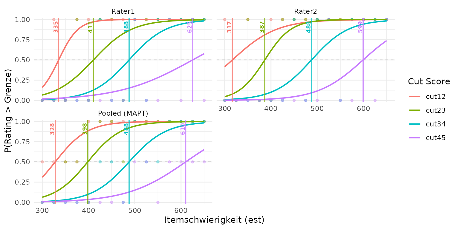
Each rater panel shows the fitted probability that a rating index
exceeds a boundary, on a zero-to-one scale. The horizontal line at 0.5
marks the cut criterion; vertical lines show the resulting
difficulty-scale cuts. The curves are solid within each panel’s observed
difficulty range and dotted outside it to identify extrapolation. The
Pooled (MAPT) panel shows the models jointly fitted to all
ratings and the cuts from cuts_summary. It does not average
the individual rater cuts. With per_rater = FALSE, this is
the only panel, including when show_aggregate = FALSE.
Raw points show the empirical proportions above each boundary at each
difficulty. show_residuals = TRUE adds empirical
proportions minus fitted probabilities. Unusable models supply no curve
or cut line. The options show_smoothed,
show_item_numbers, and show_aggregate_labels
concern only the moving-average view and have no effect for MAPT
results.
The population options also work with MAPT. For example, with PVs on the same metric as the item difficulties:
plotCutsIDM(cutsMAPT, show_aggregate = TRUE,
pv_data = population, pv_cols = c("PV1", "PV2"),
weight_col = "weight")Silhouette height shows distribution shape only, not a rating
probability. Interval percentages use the cuts in their own panel; the
pooled panel uses pooled cuts. Missing cuts prevent percentage
calculation for that panel. If fitted cuts cross, set
show_percentages = FALSE to inspect the curves without
calculating interval percentages.
For a population distribution with a density axis, use
plotPopulationCutsIDM(cutsMAPT, population, pv_cols = c("PV1", "PV2"), weight_col = "weight", cut_selection = "both").
With MAPT input, cut_selection = "mean" retains its
existing argument name but selects the pooled cuts. "both"
shows individual and pooled panels, or only the pooled panel when
per_rater = FALSE.
Visual Subset Recoding
visualSubsetRecode() supports interactive inspection and
recoding of flagged subsets. For example, if a group of students was
affected by a technical issue, you can display the relevant responses
and decide whether to recode them to a value such as mci.
Because the function opens an interactive review flow, it is not
evaluated in this vignette.
subsetInfo <- data.frame(
ID = c("person100", "person101", "person102"),
datCols = c("I01", "I02", "I03")
)
datVisRec <- visualSubsetRecode(dat = preparedData, subsetInfo = subsetInfo,
ID = "ID", toRecodeVal = "mci")Export
After the data preparation is done, you can prepare the data sets for
exporting to then use them in the packages eatModel and
eatGADS.
Collapsing Data
The last step is to recode character missings to numerical types with
collapseMissings(), usually to 1, 0 or NA, but other values
are also possible. All variables need to be converted to
numeric, as well, so you can pass the data set to
eatModel afterwards.
You can use the data frame that is returned by
recodeData(), which we called datRec earlier
(dat). But its main purpose is to finish the scored data
set as it comes out of scoreData() or
automateDataPreparation().
missing.rule is a list containing information which
character missings should be converted to 0 or
NA. It has default settings, but you can adapt them if
needed. Type ?collapseMissings into your console to learn
more.
datColMis <- collapseMissings(datRec)After doing that you should have a data frame that you can now use
for further processing with the eatModel package.
Export SPSS
With writeSpss() you can create a .txt file and a SPSS
syntax file, which can then be used in SPSS. You need the four data
frames dat, values, subunits and
units, the last three are usually part of the
inputList. You also need to specify the file names and
where to save those new files.
The function creates and saves those files, but the actual return
values for this function is NULL.
Prepare for eatGADS
prep2GADS converts the data frame that we prepared to an
eatGADS object for further use in the package eatGADS. It
uses the meta data stored in inputList, so it needs the
inputList as an argument, as well as our data frame
dat, that we have been preparing.
Here you can see two examples for creating eatGADS objects. The first
example exports scored data (trafoType = “scored”), which
usually has 0/1 values and mistypes like mbi/mbo etc. The second example
exports the raw data (trafoType = “raw”), including the
original values and subunits.
data(inputDat)
data(inputList)
# for GADSobj1
prepDatScored <- automateDataPreparation(inputList = inputList, datList = inputDat,
readSpss = FALSE, checkData=FALSE, mergeData = TRUE, recodeData=TRUE,
aggregateData=TRUE, scoreData=TRUE, writeSpss=FALSE, verbose = TRUE)
# for GADSobj2
prepDatRaw <- automateDataPreparation(inputList = inputList, datList = inputDat,
readSpss = FALSE, checkData=FALSE, mergeData = TRUE,
recodeData=FALSE, aggregateData=FALSE, scoreData=FALSE,
writeSpss=FALSE, verbose = TRUE)
GADSobj1 <- prep2GADS(dat = prepDatScored, inputList = inputList[1:3], trafoType = "scored",
                      verbose=TRUE)
#>
#> ── Check: Variables without info
#> ℹ The following 1 variable is not in inputList ($units$unit) but in dataset,
#> its meta data will be set to NA: `hisei`

GADSobj2 <- prep2GADS(dat = prepDatRaw, inputList = inputList[1:3], trafoType = "raw",
                      verbose=TRUE)
#>
#> ── Check: Variables without info
#> ℹ The following 1 variable is not in inputList ($subunits$subunit or
#> $units$unit) but in dataset, its meta data will be set to NA: `hisei`