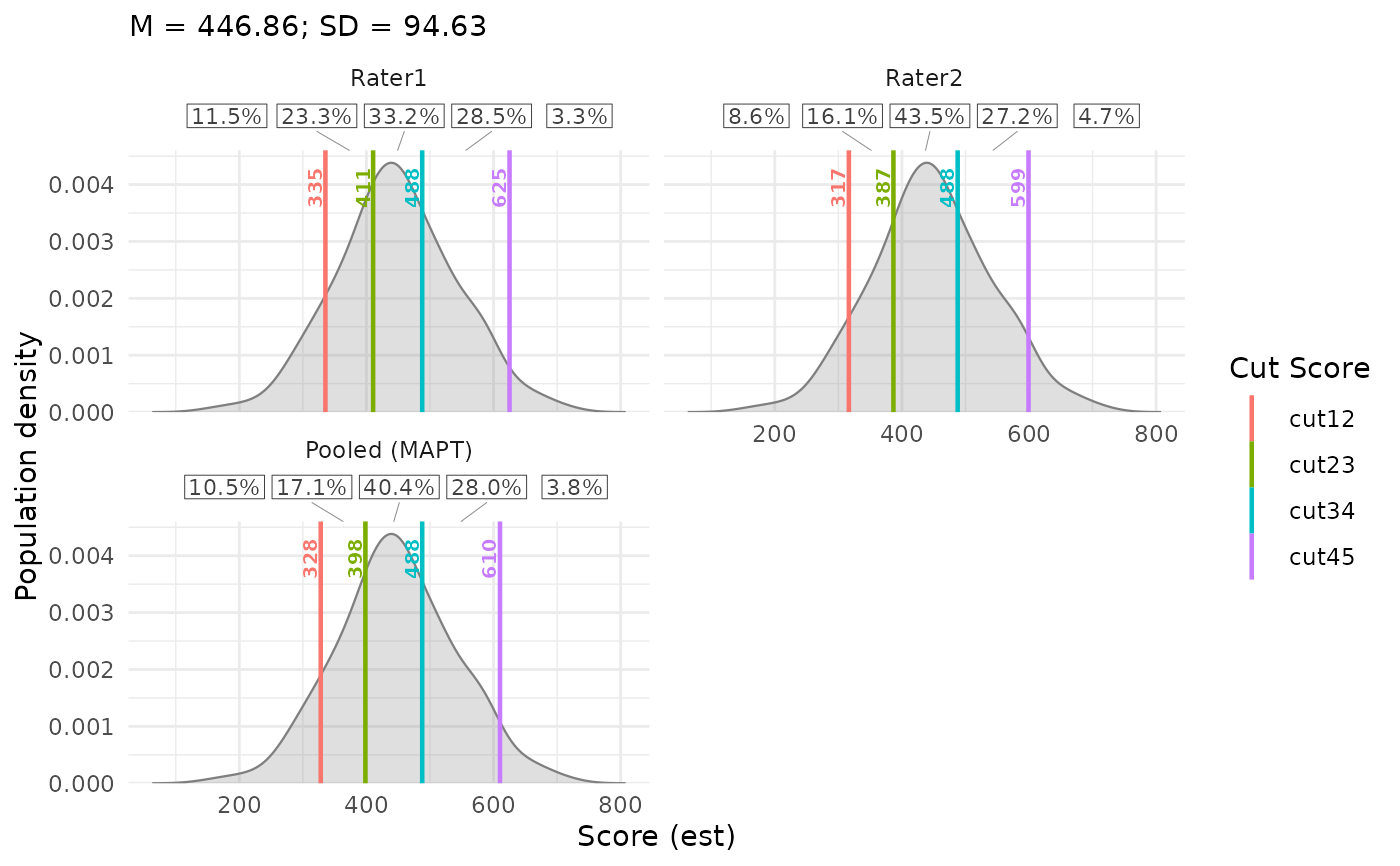
Plot Population Distributions from Plausible Values with IDM Cuts

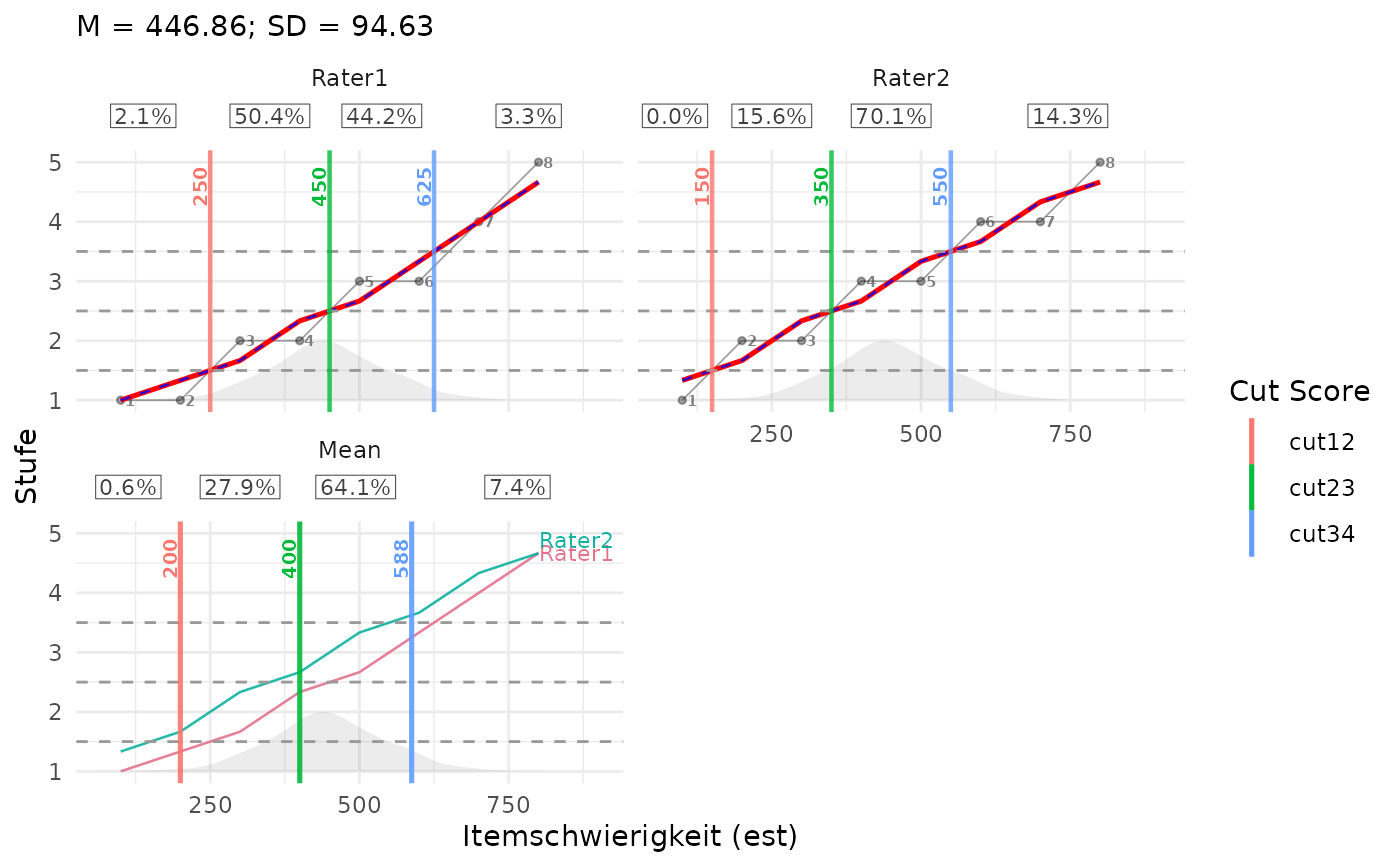
Estimates a population density from wide- or long-format plausible values (PVs) and draws IDM cut scores over it. An optional grouping column overlays multiple population densities with transparent fills. The y-axis represents population density. For a distribution-shape silhouette behind rater curves, use plotCutsIDM. For a supplied numeric cut vector without an IDM object, use plotPopulationCuts.

Usage

plotPopulationCutsIDM(
  res_list,
  pv_data,
  pv_cols = NULL,
  respondent_id_col = NULL,
  pv_id_col = NULL,
  pv_value_col = NULL,
  weight_col = NULL,
  input_format = c("auto", "long", "wide"),
  pv_missing = c("error", "drop"),
  density_bw = NULL,
  density_adjust = 1,
  cut_selection = c("mean", "individual", "both"),
  est_col = NULL,
  show_cut_values = TRUE,
  cut_value_digits = 0L,
  cut_value_size = 2.6,
  population_fill = "grey50",
  population_alpha = 0.25,
  population_col = NULL,
  population_colors = NULL,
  show_percentages = TRUE,
  percentage_digits = 1L,
  percentage_size = 3,
  show_population_stats = TRUE,
  population_stats_digits = 2L,
  show_caption = FALSE
)

Arguments

res_list: A list returned by computeCutsIDM. Cut scores are used as stored, without re-estimation.
pv_data: A data frame of plausible values for one domain, optionally containing several populations identified by population_col. PVs must already use the same metric as the item estimates and cuts. No scale conversion is performed.
pv_cols: Character vector of PV column names for wide input, with one row per respondent. Required for wide input; other numeric columns are never selected automatically.
respondent_id_col: Optional respondent ID column for wide input; required for long input. Wide IDs must be unique within each population. The same ID may occur in different populations. IDs are population respondent identifiers, not rater or item identifiers.
pv_id_col: PV identifier column for long input, for example a column containing "PV1", "PV2", and so on. Required together with pv_value_col and respondent_id_col. Each respondent-PV combination must be unique within its population.
pv_value_col: Numeric PV value column for long input.
weight_col: Optional numeric sampling-weight column. Default NULL uses equal weights. Weights must be finite, non-missing, non-negative, and constant across PVs for each respondent within a population. Zero-weight observations are excluded.
input_format: Input layout. "auto" selects long format when pv_id_col or pv_value_col is supplied, and wide format otherwise. Supply only the column selectors for the chosen layout.
pv_missing: Missing-PV policy. Default "error" rejects NA/NaN values and omitted respondent-PV rows. "drop" omits these with a warning and renormalizes weights separately within each PV. Infinite PVs and missing or invalid weights always cause an error. Every PV must retain at least two observed respondents with positive weights.
density_bw: Optional positive finite numeric bandwidth in score units. When NULL, average the unweighted stats::bw.nrd0() bandwidths across PVs within each population after exclusions, then average those population means. This common bandwidth is used for every population and PV; automatic bandwidth selection does not account for sampling weights.
density_adjust: Positive finite multiplier for the common bandwidth. Values above one produce more smoothing; values below one produce less.
cut_selection: "mean" (default) draws cuts from res_list$cuts_summary. "individual" creates one facet per rater with cuts from res_list$cuts_per_person. "both" adds a mean-cut facet to the individual facets. All facets show the same population density on fixed axes.
est_col: Optional x-axis metric label. Defaults to res_list$est_col, or "est" if unavailable. This changes the label only.
show_cut_values: Logical scalar. Show numeric labels next to finite cut lines.
cut_value_digits: Non-negative integer scalar. Digits after the decimal point for rounding cut labels; trailing zeros are removed. Default 0L.
cut_value_size: Finite non-negative cut-label text size in millimetres. Default 2.6.
population_fill: Character vector of density fill and outline colors. An explicitly supplied single color applies to all populations. Otherwise supply exactly one color per observed population, in order of first appearance in the data (the population legend order); vector names are ignored. Too few or too many colors, including an empty vector, trigger a warning and restore the default colors. If omitted, ungrouped input uses "grey50"; grouped input uses the automatic palette described under population_colors. Explicit population_colors takes precedence.
population_alpha: Finite fill opacity between zero and one. Default 0.25.
population_col: Optional grouping column identifying populations in wide or long input. Labels must be non-missing and non-empty. Groups are drawn and listed in their order of first appearance; unused factor levels are ignored. Default NULL treats all rows as one population and preserves the ungrouped plot.
population_colors: Optional named character vector of colors, with exactly one name matching each observed population label. Requires population_col and takes precedence over population_fill. With neither color argument supplied, grouped input uses blue and orange for two groups (blue for one), or a qualitative palette for more groups. A separate fill legend identifies populations; cut colors keep their existing meaning.
show_percentages: Logical scalar. Default TRUE adds a percentage table at the top of each panel. Each population has a colored row, in population-legend order. FALSE hides the table and its additional caption.
percentage_digits: Integer scalar from zero to ten. Decimal places shown in percentage labels. Default 1L. Rounding is for display only and can make displayed totals differ slightly from 100 percent.
percentage_size: Finite non-negative text size in millimetres for the percentage table. Default 3. For many intervals or small figures, reduce this size or increase the figure width.
show_population_stats: Logical scalar. Default TRUE displays the estimated mean (M) and standard deviation (SD) below each population name in the fill legend. For ungrouped data, they appear in the subtitle. FALSE hides these statistics and their explanatory caption line independently of show_percentages.
population_stats_digits: Integer scalar from zero to ten. Decimal places in displayed M and SD values. Default 2L. Legend and subtitle text sizes can be adjusted with the corresponding ggplot2::theme() settings.
show_caption: Logical scalar. Default FALSE hides explanatory plot captions. Set to TRUE to explain the density and, when displayed, percentages and M/SD below the plot. Does not affect statistics, percentage labels, or the subtitle.

Details

A Gaussian kernel density is estimated separately for each PV, using sampling weights normalized to sum to one within that PV. These densities are averaged with equal weight across PVs. All estimates use a common bandwidth and a shared grid extending three bandwidths beyond the observed PV range. The grid has at least 512 points and becomes finer when needed to resolve the bandwidth. Smoothing settings requiring excessive grid resolution cause an error; increase density_bw or density_adjust in that case. Respondents' PVs are never averaged before estimating the distribution. The automatic bandwidth is based on the respondent count within each PV, not on the number of stacked PV observations.

With population_col, PV preparation, missing-data checks, and weight normalization are performed separately within each population. Each population's density averages its own PV densities and has total area one; the plotted height is not proportional to population sample size or the sum of its weights. All populations share the same bandwidth and grid spanning their combined PV range. The automatic bandwidth gives equal weight to each population's mean PV bandwidth, including when populations have different numbers of PVs in long input. Missing-data requirements apply within each population; a PV identifier entirely absent from a population's long input cannot be detected.

Filled densities overlap without stacking, with separate colored outlines. population_alpha controls their transparency. Named colors can be reused in both plotting functions to keep the population colors consistent. Cut lines are drawn over the densities, and all selected rater/mean facets repeat the same set of distributions on fixed axes.

With show_population_stats = TRUE, M and SD are calculated from the observed PVs and sampling weights, separately within each population and PV. For each PV, normalize weights to sum to one, compute its weighted mean, and multiply the weighted mean squared deviation by $n_j/(n_j-1)$ before taking the square root. Here $n_j$ is the number of observed respondents with positive weights in that PV and population, after missing-data handling. The displayed M averages the PV means; the displayed SD is the square root of the average PV variance: $SD = \sqrt{m^{-1}\sum_{j=1}^{m} SD_j^2}$, where $m$ is the number of PVs. Every PV has equal weight. No variance component for differences between PV means is added. This estimates population SD with an $n_j/(n_j-1)$ variance correction; it is not a standard error. Respondents' PVs are never averaged before computing these statistics. With pv_missing = "drop", each PV uses its own available observations and renormalized weights. Zero-weight observations are excluded. Both statistics use the supplied score metric and are independent of cuts, zooming, density bandwidth, and cut selection. They are computed before kernel smoothing, so SD is not derived from the smoothed density curve. All facets share these population statistics; the mean-cut panel does not alter them.

With show_percentages = TRUE, shares are computed directly from the PV observations, independently of density estimation. For each population and PV, sum the sampling weights in each cut interval and divide by the total available weight for that population and PV. Multiply by 100 and average these percentages equally across PVs. Respondents' PVs are never averaged before classification. Without weight_col, observations have equal weight. With pv_missing = "drop", each denominator uses the available observations separately for its population and PV.

For cuts $c_1, \ldots, c_K$, intervals are $(-\infty, c_1)$, $[c_1, c_2)$, through $[c_K, \infty)$. A value exactly on a cut enters the upper interval. Identical adjacent cuts create an empty interval with zero percent. All observed PVs are included, including values outside the visible plot range. Actual unrounded cuts determine membership: changing cut-label rounding or density smoothing does not change percentages. Individual panels use their rater's cuts. The mean panel recomputes shares at the mean cuts; it does not average rater percentages.

Percentage labels are horizontally centered between the visible cut positions. For outer intervals, the midpoint between the outermost cut and the visible panel edge is used. Narrow or empty intervals retain their labels: overlapping labels are shifted as little as possible while preserving their order, with thin lines connecting shifted columns to their interval midpoints. Population rows share the same horizontal positions. Placement is recalculated at drawing time using the actual text widths, including after zooming or reversing the score axis. Intervals wholly outside a zoomed view are anchored at its edge; zooming does not change their percentages. Rows follow population-legend order and colors; ungrouped data have one neutral row. The table occupies a separate band above the data, with height determined by its text size and number of rows. It does not change the data axes or overlap curves when the figure is resized. Increase figure height for many panels or populations, and figure width for many intervals. If the combined label widths exceed the panel width, text and padding are reduced together to fit; increase figure width to retain the requested text size. If a panel has any missing or infinite cut, its percentage table is replaced with an explanatory message and a warning identifies the panel. Descending cut sequences cause an error when percentages are enabled.

Percentage labels are estimated population shares. Unlike these numeric labels, silhouette height in plotCutsIDM() communicates distribution shape only, not rating stages or readable density-axis values.

These are descriptive point estimates without confidence intervals or replicate-weight variances. Sampling weights affect the estimated density, but not the automatic bandwidth rule. An explicit density_bw can be supplied when a different smoothing choice is needed. With pv_missing = "drop", different PVs may use different respondent subsets; missing cases are not imputed. A PV entirely absent from long input cannot be detected, so include every intended PV identifier in the input.

PVs and cuts are drawn directly on their supplied score metric. The x-range includes the density grid and all finite selected cuts. The density is repeated unchanged across rater and mean facets; it is not conditioned on the rater.

Here the y-axis is population density. In contrast, the optional background in plotCutsIDM() is a silhouette showing distribution shape only: its height is scaled for display and does not represent rating stages or density-axis values. Use this standalone plot when the density axis matters. Both functions use the same population preparation and density calculation.

Value

A ggplot2 object that can be customized with standard ggplot layers and themes.

References

OECD, PISA Research Documentation: How to prepare and analyse the PISA database. https://www.oecd.org/en/about/programmes/pisa/how-to-prepare-and-analyse-the-pisa-database.html

Examples

items <- data.frame(
  est = seq(100, 800, by = 100),
  Rater1 = c(1, 1, 2, 2, 3, 3, 4, 5),
  Rater2 = c(1, 2, 2, 3, 3, 4, 4, 5)
)
cuts <- computeCutsIDM(items, boundaries = c(1.5, 2.5, 3.5))

## Synthetic PVs on the same score metric as the item estimates and cuts.
set.seed(42)
population <- data.frame(
  student = seq_len(200),
  PV1 = rnorm(200, 450, 100),
  PV2 = rnorm(200, 450, 100),
  weight = runif(200, 0.5, 2)
)

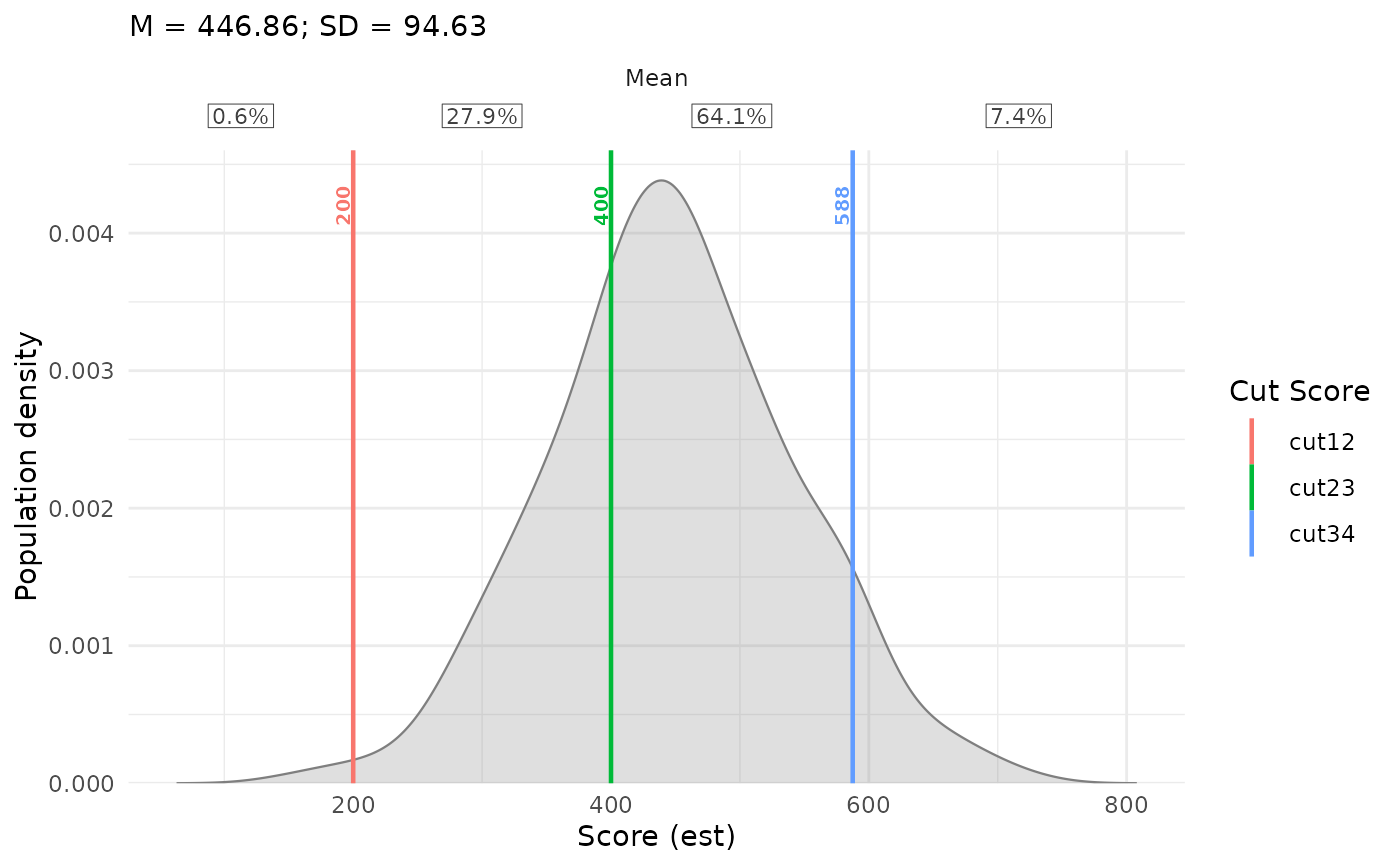
## Standalone density with mean cuts: the y-axis represents density.
plotPopulationCutsIDM(cuts, population, pv_cols = c("PV1", "PV2"),
                      weight_col = "weight")


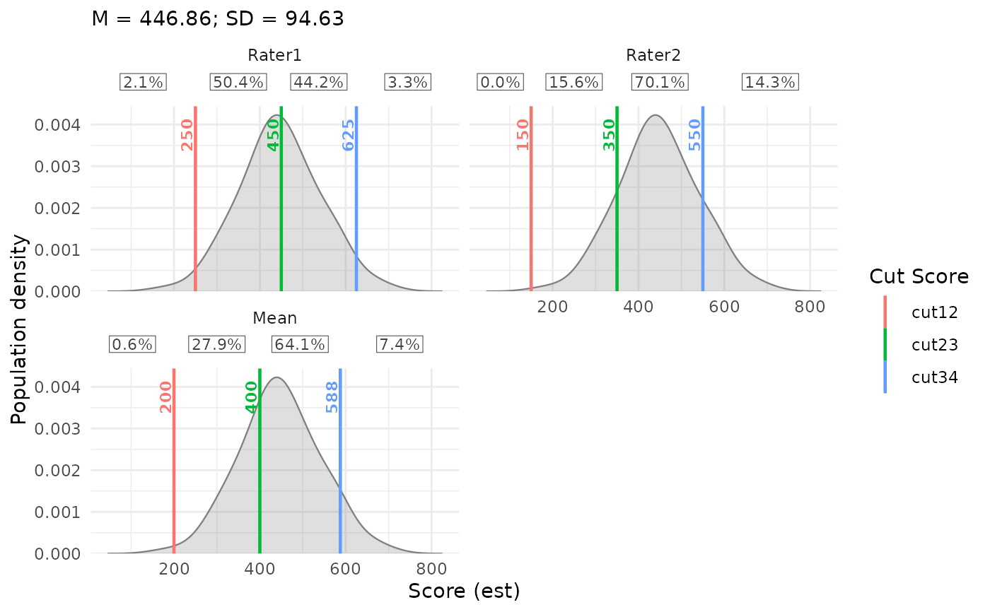
## Compare individual and mean cuts over the same population distribution.
plotPopulationCutsIDM(cuts, population, pv_cols = c("PV1", "PV2"),
                      weight_col = "weight", cut_selection = "both",
                      density_adjust = 1.2, cut_value_size = 3)


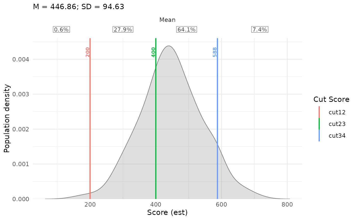
## Equivalent long input: one row per respondent and PV.
population_long <- tidyr::pivot_longer(
  population, cols = c("PV1", "PV2"),
  names_to = "pv", values_to = "score"
)
plotPopulationCutsIDM(cuts, population_long,
                      respondent_id_col = "student",
                      pv_id_col = "pv", pv_value_col = "score",
                      weight_col = "weight")


## Background silhouette: distribution shape only.
## Its height does NOT represent rating stages or density-axis values.
plotCutsIDM(cuts, pv_data = population, pv_cols = c("PV1", "PV2"),
            weight_col = "weight", show_aggregate = TRUE,
            population_height = 0.25, population_alpha = 0.15)


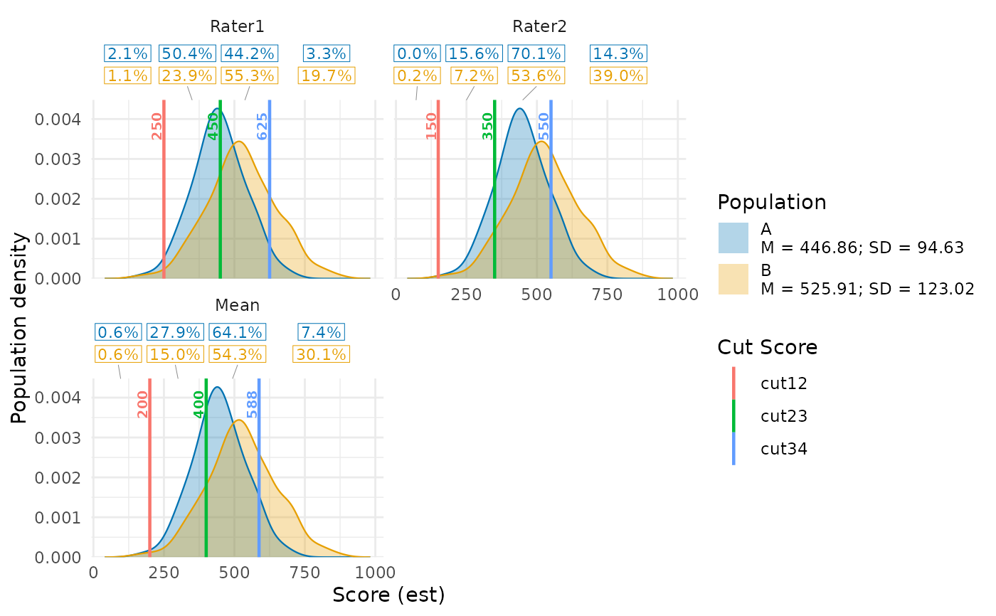
## Compare two populations; student IDs may repeat between populations.
population$group <- "A"
population_b <- population
population_b$group <- "B"
population_b[c("PV1", "PV2")] <- 450 +
  1.3 * (population_b[c("PV1", "PV2")] - 450) + 80
populations <- rbind(population, population_b)
colors <- c(A = "#0072B2", B = "#E69F00")
plotPopulationCutsIDM(cuts, populations, pv_cols = c("PV1", "PV2"),
                      respondent_id_col = "student", weight_col = "weight",
                      population_col = "group", population_colors = colors,
                      population_alpha = 0.3, cut_selection = "both")


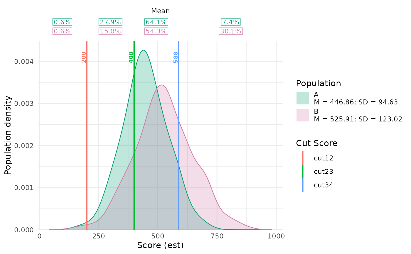
## Alternatively, supply fill colors in population legend order.
plotPopulationCutsIDM(cuts, populations, pv_cols = c("PV1", "PV2"),
                      weight_col = "weight", population_col = "group",
                      population_fill = c("#009E73", "#CC79A7"))

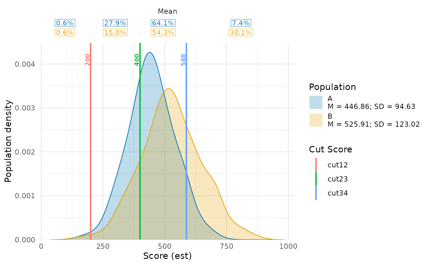
## A single population_fill color would apply to both groups.
## Three colors for these two groups would warn and restore the default palette.

## Equivalent grouped long input.
populations_long <- tidyr::pivot_longer(
  populations, cols = c("PV1", "PV2"), names_to = "pv", values_to = "score"
)
plotPopulationCutsIDM(cuts, populations_long, respondent_id_col = "student",
                      pv_id_col = "pv", pv_value_col = "score", weight_col = "weight",
                      population_col = "group", population_colors = colors)


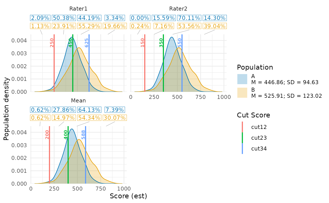
## Percentages use actual panel cuts, independently of density smoothing.
plotPopulationCutsIDM(cuts, populations, pv_cols = c("PV1", "PV2"),
                      weight_col = "weight", population_col = "group",
                      cut_selection = "both", percentage_digits = 2,
                      percentage_size = 3.5)


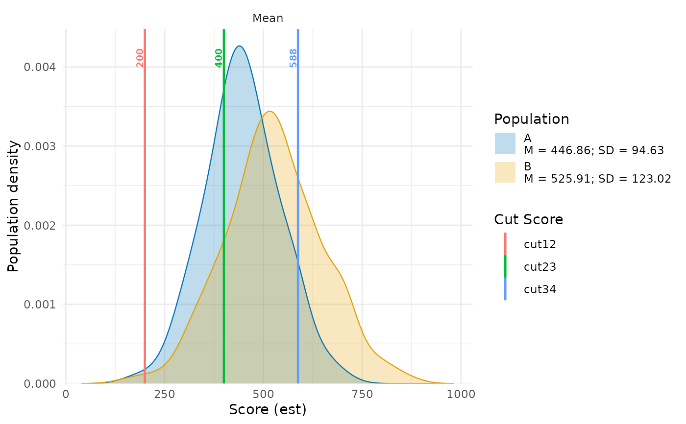
## Hide percentage tables, keeping the density and numeric cut labels.
plotPopulationCutsIDM(cuts, populations, pv_cols = c("PV1", "PV2"),
                      weight_col = "weight", population_col = "group",
                      show_percentages = FALSE)


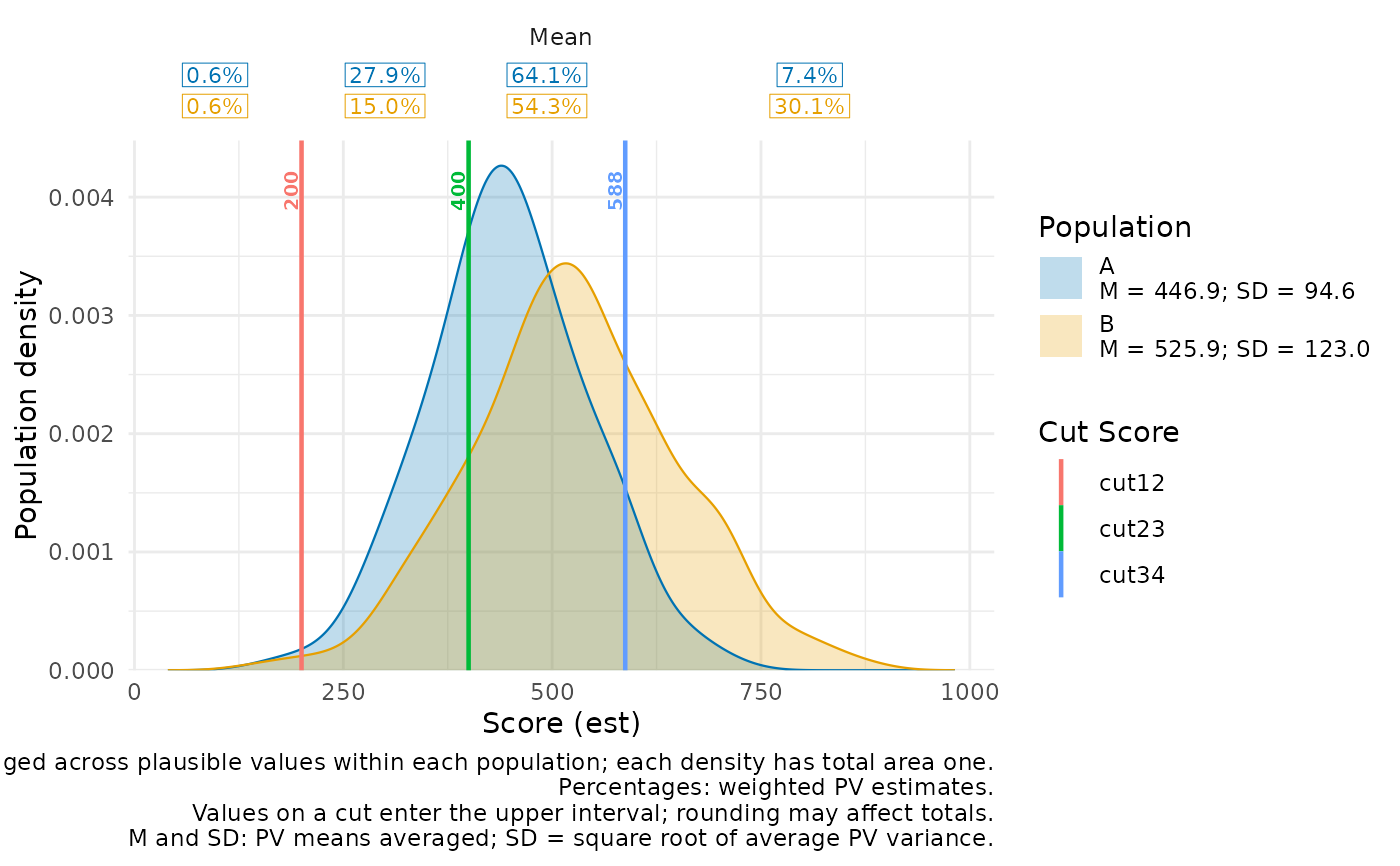
## Format M and SD in the population legend, independently of percentages.
plotPopulationCutsIDM(cuts, populations, pv_cols = c("PV1", "PV2"),
                      weight_col = "weight", population_col = "group",
                      population_stats_digits = 1, show_caption = TRUE)


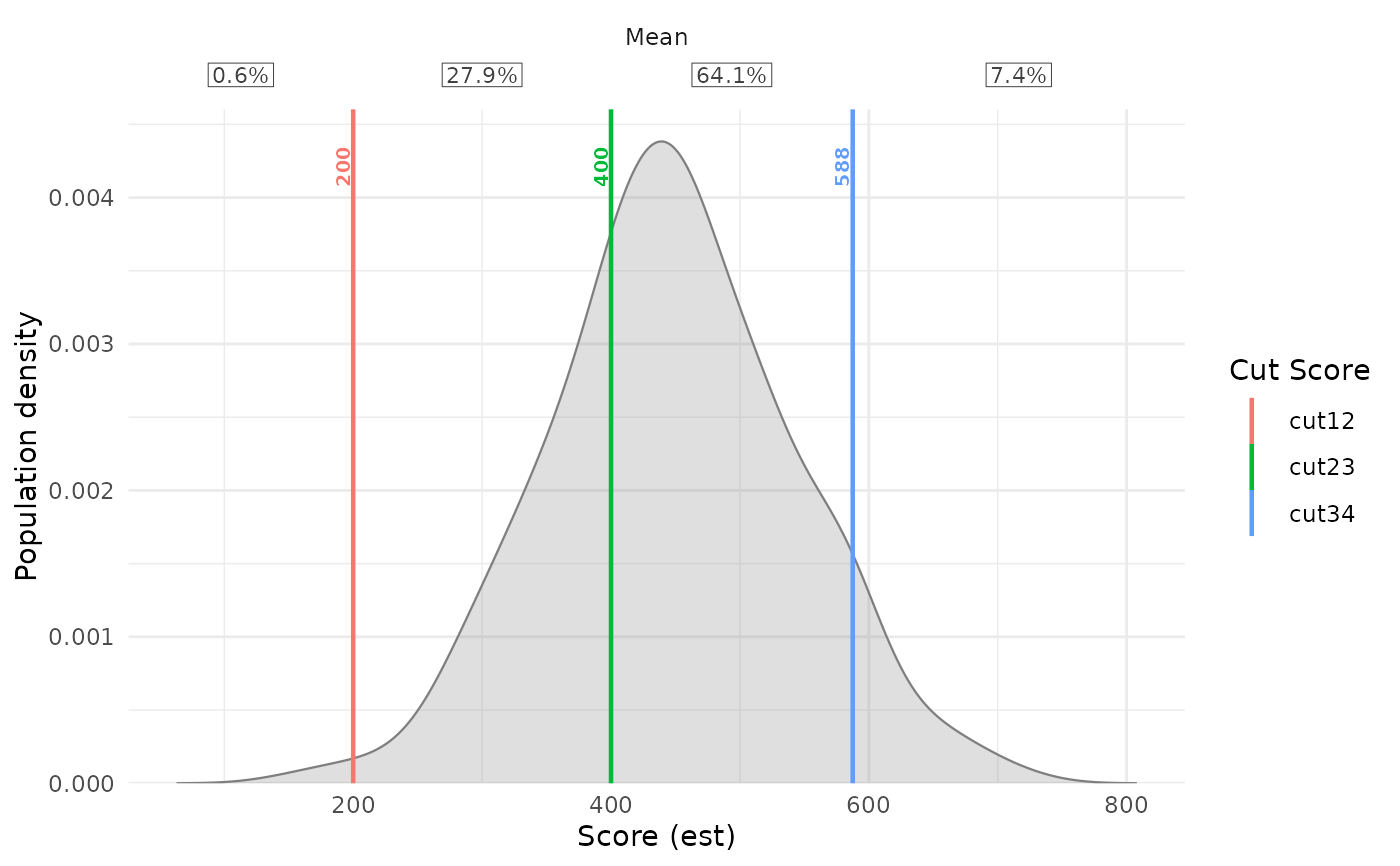
## Hide M and SD while keeping the cut-interval percentages.
plotPopulationCutsIDM(cuts, population, pv_cols = c("PV1", "PV2"),
                      weight_col = "weight", show_population_stats = FALSE)