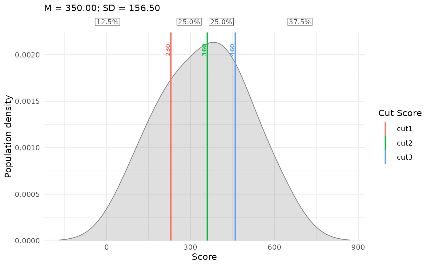
Plot Population Distributions with Supplied Cut Scores

Plots a population density estimated from plausible values (PVs), with supplied numeric cut scores and percentage shares for the resulting intervals. No IDM result object is needed. Supports the same PV layouts, weights, population groups, and display options as plotPopulationCutsIDM.

Usage

plotPopulationCuts(
  cuts, pv_data, pv_cols = NULL,
  respondent_id_col = NULL,
  pv_id_col = NULL, pv_value_col = NULL,
  weight_col = NULL,
  input_format = c("auto", "long", "wide"),
  pv_missing = c("error", "drop"),
  density_bw = NULL, density_adjust = 1,
  cut_labels = NULL, est_col = NULL,
  show_cut_values = TRUE,
  cut_value_digits = 0L, cut_value_size = 2.6,
  population_fill = "grey50", population_alpha = 0.25,
  population_col = NULL, population_colors = NULL,
  show_percentages = TRUE, percentage_digits = 1L,
  percentage_size = 3,
  show_population_stats = TRUE, population_stats_digits = 2L,
  show_caption = FALSE
)

Arguments

cuts: Non-empty, finite numeric vector of strictly increasing cut scores, on the same scale as the PVs. Missing, duplicate, or unsorted cuts are rejected. Vector names are ignored; use cut_labels to label the cut lines.
pv_data: Data frame of plausible values for one domain, optionally containing multiple populations. No scale conversion is performed.
pv_cols: Explicit character vector of PV columns for wide input, with one row per respondent. Required for wide input.
respondent_id_col: Optional respondent ID column for wide input; required for long input. IDs must be unique within each population in wide input.
pv_id_col: PV identifier column for long input. Each respondent-PV combination must be unique within its population.
pv_value_col: Numeric PV value column for long input.
weight_col: Optional numeric sampling-weight column. Weights must be finite, non-missing, non-negative, and constant across each respondent's PVs. Zero-weight observations are excluded. Default NULL uses equal weights.
input_format: "auto" selects long input when pv_id_col or pv_value_col is supplied, and wide input otherwise.
pv_missing: "error" rejects missing PV values or respondent-PV rows. "drop" omits them with a warning and renormalizes weights within each PV and population. Each PV requires at least two observed respondents with positive weights. Infinite PVs and invalid weights always cause an error.
density_bw: Optional positive finite bandwidth in score units. The default averages unweighted stats::bw.nrd0() bandwidths across PVs within populations, then across populations. See plotPopulationCutsIDM.
density_adjust: Positive finite multiplier for the common bandwidth.
cut_labels: Optional character vector with one unique, non-empty label per cut, in cut order. Defaults to "cut1", "cut2", etc. These label cut lines in the legend, not intervals.
est_col: Optional x-axis metric label. Default NULL labels the axis "Score"; otherwise the label is "Score (<est_col>)".
show_cut_values: Show numeric labels next to cut lines.
cut_value_digits: Non-negative integer number of decimal places in cut labels. Trailing zeros are removed. This does not change interval membership.
cut_value_size: Non-negative cut-label text size in millimetres.
population_fill: Density fill and outline color, or one color per population in order of first appearance. If omitted, grouped input uses an automatic palette. An incorrect color count warns and restores defaults.
population_alpha: Fill opacity between zero and one.
population_col: Optional grouping column. Population identifiers must be non-missing and non-empty. Densities and percentages are estimated separately within each population, in order of first appearance.
population_colors: Optional named color vector with exactly one color for each population. Requires population_col; takes precedence over population_fill.
show_percentages: Show interval percentages above the density panel. Hiding labels does not suppress the returned percentage table.
percentage_digits: Integer from zero to ten specifying decimal places in displayed percentages. Rounding may make displayed totals differ from 100.
percentage_size: Non-negative percentage text size in millimetres.
show_population_stats: Show population mean and SD in the population legend, or subtitle for ungrouped input.
population_stats_digits: Integer from zero to ten specifying decimal places in displayed mean and SD.
show_caption: Show explanatory captions. Defaults to FALSE.

Details

Gaussian kernel densities are estimated separately for each PV using normalized sampling weights, then averaged equally across PVs. Populations share a common bandwidth and grid, and each density has area one. PVs are never averaged within respondents before estimation.

Percentages are computed directly from observed PVs, independently of density smoothing. For each population and PV, the weights in each interval are divided by that PV's total available weight and multiplied by 100. These percentages are then averaged equally across PVs. With cuts \(c_1, \ldots, c_K\), intervals are \((-\infty, c_1)\), \([c_1, c_2)\), through \([c_K, \infty)\). Equality belongs to the upper interval. All available values contribute, including values outside the visible plot range. Missing-value dropping renormalizes weights within each PV and population.

Population means average the per-PV weighted means. SD is the square root of the average per-PV variance, with the \(n/(n-1)\) correction applied within each PV and population. See plotPopulationCutsIDM for details of estimation, missing-data handling, colors, and percentage-label placement.

Value

A ggplot object that can be printed, customized, or saved with ggplot2::ggsave(). Its "population_percentages" attribute is a data frame with columns population, interval (starting at one), lower, upper, and percentage (unrounded, from zero to 100). Outer bounds are infinite. Ungrouped input uses the population label "Population". The table is calculated even if show_percentages = FALSE. Extract it with attr(p, "population_percentages") before further plot customization. These are descriptive shares, without standard errors.

Examples

pvs <- data.frame(
  PV1 = c(100, 230, 360, 460),
  PV2 = c(230, 360, 460, 600),
  weight = c(1, 2, 3, 4)
)
p <- plotPopulationCuts(
  cuts = c(230, 360, 460), pv_data = pvs,
  pv_cols = c("PV1", "PV2"), weight_col = "weight"
)
p

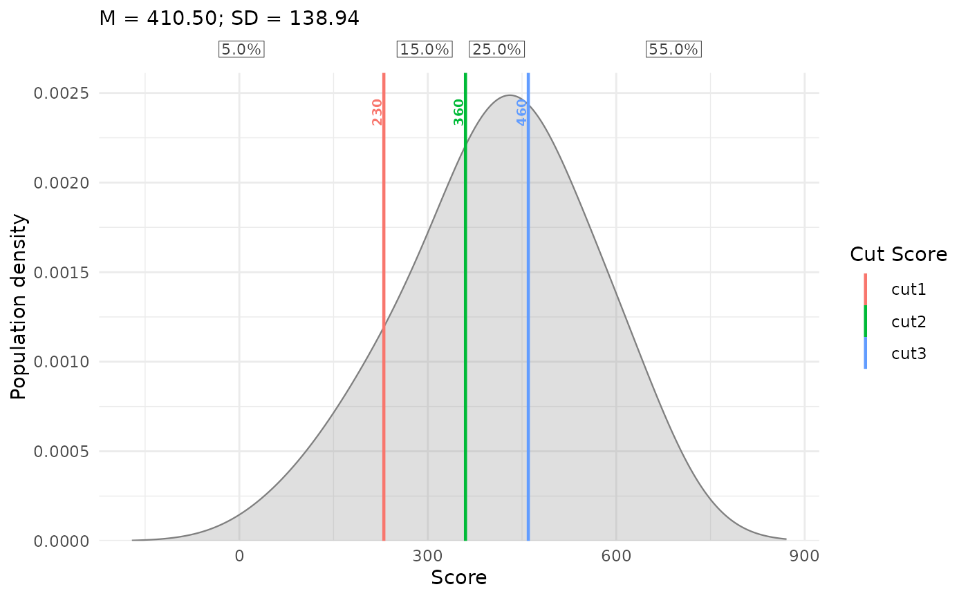attr(p, "population_percentages")
#>   population interval lower upper percentage
#> 1 Population        1  -Inf   230          5
#> 2 Population        2   230   360         15
#> 3 Population        3   360   460         25
#> 4 Population        4   460   Inf         55

long_pvs <- data.frame(
  id = rep(1:4, times = 2), pv = rep(c("PV1", "PV2"), each = 4),
  score = c(pvs$PV1, pvs$PV2)
)
plotPopulationCuts(
  c(230, 360, 460), long_pvs,
  respondent_id_col = "id", pv_id_col = "pv", pv_value_col = "score"
)